
Hands-on Tutorials
Seeing patterns in data is great, but using data to intervene and ask "what if" is next-level. You'll be surprised how easily do-calculus lets you interrogate your dataset with real causal confidence.
With the rise of Large Language Models (LLMs), it has become possible to "ask questions" to your data set. Although this is powerfull, an approach with LLMs also has major drawbacks, especially when using it in automated pipelines or high-impact decision processes. To maintain control and ensure accuracy, we can turn to Bayesian inference. This blog walks you through how to learn Bayesian models and demonstrates how to apply do-calculus to an example data set. You will be surprised by how easily you can build models that let you chat with your data using the bnlearn library.
If you found this article helpful, you are welcome to follow me because I write more about Bayesian statistics! I recommend experimenting with the hands-on examples in this blog. This will help you to learn quicker, understand better, and remember longer. Grab a coffee and have fun!
A Brief Introduction: Asking Questions To Data Sets.
For decades, we dreamed of having an intuitive interface where a data set could simply be dropped into a system and queried directly. However, when using statistics, it is more common to first formulate hypotheses before doing the analysis. This is a process that can be rigid and slow, as there are many intermediate steps. With the rise of Large Language Models (LLMs), this long-standing dream finally feels within reach. Using natural language (typed or spoken), LLMs can automatically generate queries or Python code. You can now upload a data set with for example the salaries of data scientists and instantly ask, "What was the average salary of data scientists in Europe last year?". Without writing a single line of code, the answer will be returned. More details about building your (local) LLMs and their usage can be found in this blog:
The ability to interogate data sets has always been an intriguing prospect for researchers and practitioners.
However, this new power comes with a trade-off: a significant loss of transparency and control. LLMs are deep black boxes; it is not always transparent why a specific query was generated or how a particular conclusion was reached. This lack of explainability is a major drawback when we need to understand the causal mechanisms within our data. This need for clarity becomes absolutely critical when model outcomes are used in high-impact processes, such as medical diagnoses, financial investments, or operational changes. We thus need a way to marry the intuitive, "conversational" interface with a more rigorous, transparent, and causal power of formal statistical methods. This is where Bayesian inference and causal networks come into play!
In the next sections, we will go through the steps of building a transparent Bayesian network to analyze a mixed data set. Then we will apply do-calculus to effectively and rigorously query it. Keep on reading to discover how Bayesian frameworks allow you to interact with data sets while maintaining full control.
The BNLearn library for Python.
A few words about the bnlearn library that is used for all the analyses in this blog: the bnlearn for Python library provides tools for creating, analyzing, and visualizing Bayesian networks in Python. It supports discrete, mixed, and continuous datasets and is designed to be easy to use while including the most essential Bayesian pipelines for causal learning. With bnlearn, you can perform structure learning, parameter estimation, inference, and create synthetic data, making it suitable for both exploratory analysis and advanced causal discovery. A range of statistical tests can be applied simply by specifying parameters during initialization. Additional helper functions allow you to transform datasets, derive the topological ordering of an entire graph, compare two networks, and generate a wide variety of insightful plots. Core functionalities include:
The key pipelines are:
- Structure Learning: Learn the network structure from data or integrate expert knowledge.
- Parameter Learning: Estimate conditional probability distributions from observed data.
- Inference: Query the network to compute probabilities, simulate interventions, and test causal effects.
- Synthetic Data: Generate new datasets from learned Bayesian networks for simulation, benchmarking, or data augmentation.
- Discretize Data: Transform continuous variables into discrete states using built-in discretization methods for easier modeling and inference.
- Model Evaluation: Compare networks using scoring functions, statistical tests, and performance metrics.
- Visualization: Interactive graph plotting, probability heatmaps, and structure overlays for transparent analysis.
What benefits does bnlearn offer over other Bayesian analysis implementations?
- Contains the most-wanted Bayesian pipelines.
- Simple and intuitive in usage.
- Open-source with MIT Licence.
- Documentation page and blogs.
- +500 stars on GitHub with over 600K downloads.
Bnlearn thus provided numerous functions and helper utilities to assist users throughout the analysis process. These include data set transformation functions, topological ordering derivation, graph comparison tools, insightful interactive plotting capabilities, and more. The bnlearn library also supports loading BIF files, converting directed graphs to undirected ones, and performing statistical tests to assess independence among variables. If you want to see a comparison between various causal models, I recommend reading this blog:
In the next section, we will jump into making inferences using do-calculus with hands-on examples. This allows you to ask questions to your data set. As mentioned earlier, structure learning and parameter learning form the basis.
Do-Calculus: Interrogating Data Sets.
When we make inferences using do-calculus, it simply means that we can query the data set and "ask questions" to it. This approach is different then when using regular statistics such as associations or correlations. With regular statistics, we can answer questions based on existing records, like "What's the average salary for developers with certification in Python?". This is what we call passive observation.
With Do-calculus (by Judea Pearl), we can move beyond passive observation. Judea Pearl provided the mathematical framework to rigorously answer causal questions and interventions. It lets us ask: "What would the average salary become if we did enforce certification of Python for all developers?": P(Salary | do(Certification=Python)). This simulates actively changing the system.
To have knowledge on how to effectively change the system, we need two main ingredients: the Directed Acyclic Graph (DAG) and the Conditional Probability Tables (CPTs).
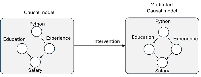
- The DAG (Directed Acyclic Graph): This is the blueprint. Its nodes represent variables (like "Education," "Experience," "Job Type," "Salary"). Its directed edges represent our explicit assumptions about causal influences (e.g., "Education → Salary", "Experience → Salary"). Crucially, the DAG encodes what variables potentially confound relationships and where interventions apply.
- CPTs (Conditional Probability Tables): For each node in the DAG, a CPT quantifies how likely its different states are, given the states of its direct parent nodes. The CPT for "Salary" contains probabilities like
P(Salary=High | Education=Masters, Experience=10+ years). These tables capture the strength and nature of the local causal dependencies defined by the graph structure.
More details about the intervention and changing the outcome using Bayesian models can be found here:
Altogether, the DAG and its CPTs form a complete causal Bayesian network while Do-calculus operates on this network. It leverages the causal assumptions encoded in the DAG to determine if (and how) the effect of an intervention (do(X)) can be estimated purely from observational data (P(Y | X, Z...)) and the structure, often by strategically adjusting for specific variables.
Let's move on and create an example where we can see how it really works. We'll build and query a causal Bayesian network using the bnlearn library on the Data Science Salary dataset. You'll discover just how intuitive "chatting" with your data via causal interventions can be.
Hands-On Do-Calculus On a Mixed Data Set.
For demonstration, we will use the data science salary data set that is derived from ai-jobs.net [5]. The salary data set is collected worldwide and contains 11 features for 4134 samples. You can load the data as shown in the code block below. Explore the columns and set features as continuous or categorical. Note that the model complexity increases with the number of categories, which means that more computation time is required to determine a causal DAG.
# Install datazets.
!pip install datazets
# Import library
import datazets as dz

# Get the data science salary data set
df = dz.get('ds_salaries')

# The features are as following
df.columns
# 'work_year'          > The year the salary was paid.
# 'experience_level'   > The experience level in the job during the year.
# 'employment_type'    > Type of employment: Part-time, full time, contract or freelance.
# 'job_title'          > Name of the role.
# 'employee_residence' > Primary country of residence.
# 'remote_ratio'       > Remote work: less than 20%, partially, more than 80%
# 'company_location'   > Country of the employer's main office.
# 'company_size'       > Average number of people that worked for the company during the year.
# 'salary'             > Total gross salary amount paid.
# 'salary_currency'    > Currency of the salary paid (ISO 4217 code).
# 'salary_in_usd'      > Converted salary in USD.
Complexity is a major limitation for Bayesian Models.
When the variables contain many categories, the complexity grows exponentially with the number of parent nodes associated with that table. In other words, when you increase the number of categories, it likely requires significantly more data to gain reliable results. Think about it like this: when you split the data into categories, the number of samples within a single category will become smaller after each split. The low number of samples per category directly affects the statistical power. In our example, we have a feature job_title that contains 99 unique titles for which 14 job titles (such as data scientists) contain 25 samples or more. The remaining 85 job titles are either unique or seen only a few times. To make sure this feature is not removed by the model because a lack of statistical power, we need to aggregate some of the job titles. In the code section below, we will aggregate job titles into 7 main categories. This results in categories that have enough samples for Bayesian modeling.
# Group similar job titles
titles = [['data scientist', 'data science', 'research', 'applied', 'specialist', 'ai', 'machine learning'],
          ['engineer', 'etl'],
          ['analyst', 'bi', 'business', 'product', 'modeler', 'analytics'],
          ['manager', 'head', 'director'],
          ['architect', 'cloud', 'aws'],
          ['lead/principal', 'lead', 'principal'],
          ]

# Aggregate job titles
job_title = df['job_title'].str.lower().copy()
df['job_title'] = 'Other'
# Store the new names
for t in titles:
    for name in t:
        df['job_title'][list(map(lambda x: name in x, job_title))]=t[0]

print(df['job_title'].value_counts())
# engineer          1654
# data scientist    1238
# analyst            902
# manager            158
# architect          118
# lead/principal      55
# Other                9
# Name: job_title, dtype: int64
The next preprocessing step is to rename some of the feature names. In addition, we will also add a new feature that describes whether the company was located in the USA or Europe, and remove some redundant variables, such as salary_currency and salary.
import numpy as np

# Rename catagorical variables for better understanding
df['experience_level'] = df['experience_level'].replace({'EN': 'Entry-level', 'MI': 'Junior Mid-level', 'SE': 'Intermediate Senior-level', 'EX': 'Expert Executive-level / Director'}, regex=True)
df['employment_type'] = df['employment_type'].replace({'PT': 'Part-time', 'FT': 'Full-time', 'CT': 'Contract', 'FL': 'Freelance'}, regex=True)
df['company_size'] = df['company_size'].replace({'S': 'Small (less than 50)', 'M': 'Medium (50 to 250)', 'L': 'Large (>250)'}, regex=True)
df['remote_ratio'] = df['remote_ratio'].replace({0: 'No remote', 50: 'Partially remote', 100: '>80% remote'}, regex=True)

# Add new feature
df['country'] = 'USA'
countries_europe = ['SM', 'DE', 'GB', 'ES', 'FR', 'RU', 'IT', 'NL', 'CH', 'CF', 'FI', 'UA', 'IE', 'GR', 'MK', 'RO', 'AL', 'LT', 'BA', 'LV', 'EE', 'AM', 'HR', 'SI', 'PT', 'HU', 'AT', 'SK', 'CZ', 'DK', 'BE', 'MD', 'MT']
df['country'][np.isin(df['company_location'], countries_europe)]='europe'
# Remove redundant variables
salary_in_usd = df['salary_in_usd']
#df.drop(labels=['salary_currency', 'salary'], inplace=True, axis=1)
As a final step, we need to discretize, salary_in_usd which can be done manually or using the discretizer function in bnlearn. For demonstration purposes, let's do both. For the latter case, we assume that salary depends on experience_level and on the country. For details, I recommend reading this blog [6]. Based on these input variables, the salary is then partitioned into bins (see code section below).
import bnlearn as bn

# Discretize the salary feature.
discretize_method='manual'

# Discretize Manually
if discretize_method=='manual':
    # Set salary
    df['salary_in_usd'] = None
    df['salary_in_usd'].loc[salary_in_usd<80000]='<80K'
    df['salary_in_usd'].loc[np.logical_and(salary_in_usd>=80000, salary_in_usd<100000)]='80-100K'
    df['salary_in_usd'].loc[np.logical_and(salary_in_usd>=100000, salary_in_usd<160000)]='100-160K'
    df['salary_in_usd'].loc[np.logical_and(salary_in_usd>=160000, salary_in_usd<250000)]='160-250K'
    df['salary_in_usd'].loc[salary_in_usd>=250000]='>250K'
else:
    # Discretize automatically but with prior knowledge.
    tmpdf = df[['experience_level', 'salary_in_usd', 'country']]
    # Create edges
    edges = [('experience_level', 'salary_in_usd'), ('country', 'salary_in_usd')]
    # Create DAG based on edges
    DAG = bn.make_DAG(edges)
    bn.plot(DAG)
    # Discretize the continous columns
    df_disc = bn.discretize(tmpdf, edges, ["salary_in_usd"], max_iterations=1)
    # Store
    df['salary_in_usd'] = df_disc['salary_in_usd']
    # Print
    print(df['salary_in_usd'].value_counts())
The Final DataFrame
The final data frame has 10 features with 4134 samples. Each feature is a categorical feature with two or multiple states. This data frame will serve as the input to learn the structure and determine the causal DAG.
# work_year           experience_level  ... country salary_in_usd
# 0          2023           Junior Mid-level  ...     USA         >250K
# 1          2023  Intermediate Senior-level  ...     USA      160-250K
# 2          2023  Intermediate Senior-level  ...     USA      100-160K
# 3          2023  Intermediate Senior-level  ...     USA      160-250K
# 4          2023  Intermediate Senior-level  ...     USA      100-160K
#     ...                        ...  ...     ...           ...
# 4129       2020  Intermediate Senior-level  ...     USA         >250K
# 4130       2021           Junior Mid-level  ...     USA      100-160K
# 4131       2020                Entry-level  ...     USA      100-160K
# 4132       2020                Entry-level  ...     USA      100-160K
# 4133       2021  Intermediate Senior-level  ...     USA       60-100K
#
# [4134 rows x 10 columns]
Bayesian Structure Learning: Estimate the DAG.
At this point, we have preprocessed the data set, and we are ready to learn the causal structure. There are six algorithms implemented in bnlearn that can help with this task. We need to choose a method that can handle categories but without the need for a target value. The most well-known search strategies are:
- The hillclimbsearch algorithm is a heuristic search method. It starts with an empty network and iteratively adds or removes edges based on a scoring metric. The algorithm explores different network structures and selects the one with the highest score.
- The exhaustivesearch performs an exhaustive search over all possible network structures to find the optimal Bayesian network. It evaluates and scores each structure based on a specified scoring metric. While this method guarantees finding the best network structure, it can be computationally expensive for large networks due to the exponential growth of possibilities.
- The constraintsearch incorporates user-specified constraints or expert knowledge into the structure learning process of a Bayesian network. It uses these constraints to guide the search and restrict the space of possible network structures, ensuring that the learned network adheres to the specified constraints.
- The chow-liu algorithm is a method for learning the structure of a tree-structured Bayesian network. It calculates the mutual information between each pair of variables and constructs a tree by greedily selecting the edges that maximize the total mutual information of the network. This algorithm is efficient and widely used for learning the structure of discrete Bayesian networks but requires setting a root node.
- The naivebayes algorithm assumes that all features in a dataset are conditionally independent given the class variable. It learns the conditional probability distribution of each feature given the class and uses Bayes theorem to calculate the posterior probability of the class given the features. Despite its naive assumption, this algorithm is often used in classification tasks and can be efficient for large datasets.
- The TAN (Tree-Augmented Naive Bayes) algorithm is an extension of the naive Bayes algorithm that allows for dependencies among the features, given the class variable. It learns a tree structure that connects the features and uses this structure to model the conditional dependencies. TAN combines the simplicity of naive Bayes with some modeling power, making it a popular choice for classification tasks with correlated features. This method requires setting a class node.
The scoring types BIC, K2, BDS, AIC, and BDEU are used to evaluate and compare different network structures. As an example, BIC balances the model complexity and data fit, while the others consider different types of prior probabilities. In addition, the independence test prunes the spurious edges from the model. In our use case, I will use the hillclimbsearch method with the scoring type BIC for structure learning. We will not define a target value but let the bnlearn decide the entire causal structure of the data itself. More details can be found in this blog:
The code block for structure learning would look like this:
# Structure learning
model = bn.structure_learning.fit(df, methodtype='hc', scoretype='bic')

# independence test
model = bn.independence_test(model, df, prune=False)
# Parameter learning to learn the CPTs. This step is required to make inferences.
model = bn.parameter_learning.fit(model, df, methodtype="bayes")

# Plot
bn.plot(model, title='Salary data set')
bn.plot(model, interactive=True, title='method=tan and score=bic')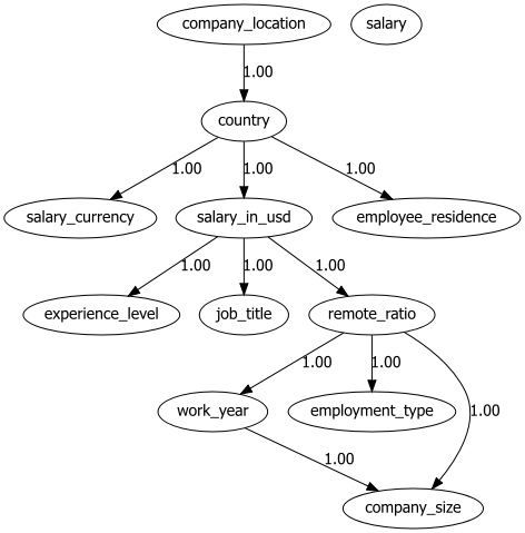
Chat With Your Data Set: Making Inferences
With the learned DAG (Figures 1 and 2), we can estimate the conditional probability distributions (CPTs, see code section below), and make inferences using do-calculus. Let's start asking questions. Note that the results can (slightly) change based on the stochastic components in the model.
Question:
What is the probability of a job title given that you work in a large comany?
P(job_title | company_size=Large (>250))
After running the code section below, we can see that the engineer is the most likely outcome (P=0.344871) followed by the data scientist (P=0.266385).
query = bn.inference.fit(model, variables=['job_title'],
                         evidence={'company_size': 'Large (>250)'})

"""
[bnlearn] >Variable Elimination.
+----+----------------+-----------+
|    | job_title      |         p |
+====+================+===========+
|  0 | Other          | 0.0310497 |
+----+----------------+-----------+
|  1 | analyst        | 0.207691  |
+----+----------------+-----------+
|  2 | architect      | 0.0508861 |
+----+----------------+-----------+
|  3 | data scientist | 0.266385  |
+----+----------------+-----------+
|  4 | engineer       | 0.344871  | <-- Highest probability
+----+----------------+-----------+
|  5 | lead/principal | 0.0402213 |
+----+----------------+-----------+
|  6 | manager        | 0.0588963 |
+----+----------------+-----------+

Summary for variables: ['job_title']
Given evidence: company_size=Large (>250)

job_title outcomes:
- job_title: Other (3.1%)
- job_title: analyst (20.8%)
- job_title: architect (5.1%)
- job_title: data scientist (26.6%)
- job_title: engineer (34.5%)
- job_title: lead/principal (4.0%)
- job_title: manager (5.9%)
"""
Question:
What is the probability of a salary range given a full time employment type, partially remote work, have the data science function at entry level and live in germany (DE)?
In the results below, we can see our five salary categories for which the strongest posterior probability P=0.77 is a salary of <80K under these conditions. Note that other salaries also occur, but they happen less frequently. By changing the variables and evidence, we can ask all kinds of questions. For example, we can now change experience level, residence, job title, etc, and determine how the probabilities are changing.
query = bn.inference.fit(model,
                         variables=['salary_in_usd'],
                         evidence={'employment_type': 'Full-time',
                                   'remote_ratio': 'Partially remote',
                                   'job_title': 'data scientist',
                                   'employee_residence': 'DE',
                                   'experience_level': 'Entry-level'})

"""
[bnlearn] >Variable Elimination.
+----+-----------------+-----------+
|    | salary_in_usd   |         p |
+====+=================+===========+
|  0 | 100-160K        | 0.0326173 |
+----+-----------------+-----------+
|  1 | 160-250K        | 0.0193029 |
+----+-----------------+-----------+
|  2 | 80-100K         | 0.105408  |
+----+-----------------+-----------+
|  3 | <80K            | 0.779638  |
+----+-----------------+-----------+
|  4 | >250K           | 0.0630333 |
+----+-----------------+-----------+

Summary for variables: ['salary_in_usd']
Given evidence: employment_type=Full-time, remote_ratio=Partially remote, job_title=data scientist, employee_residence=DE, experience_level=Entry-level

salary_in_usd outcomes:
- salary_in_usd: 100-160K (3.3%)
- salary_in_usd: 160-250K (1.9%)
- salary_in_usd: 80-100K (10.5%)
- salary_in_usd: <80K (78.0%)
- salary_in_usd: >250K (6.3%)

"""
Limitations Of Causal Inferences.
The goal of causal inference is to understand the outcome of alternative courses of action. Such as asking "what happens if we pull this lever?" but the answer always comes with the assumptions we make. Our assumptions can be more influential than in typical tasks for probabilistic modeling, and testing those assumptions is important to assess the validity of causal inference [8].
Final words.
In this blog, we explored how to move beyond simple correlations and truly "chat" with your data in a causal way. By building a Bayesian network, we created a transparent model of how variables like experience, education, and certification relate to salary. More importantly, we used do-calculus to go beyond observation and ask what if, simulating interventions and getting answers grounded in causal reasoning, not just patterns.
With tools like bnlearn, setting up such models is surprisingly straightforward, even for mixed data types. The real win, though, is clarity: every assumption is visible in the DAG, every probability can be inspected, and every query has a clear interpretation. This makes Bayesian causal models not just powerful, but trustworthy for embedding into automated pipelines where explainability and control matter. So next time you want to ask your data a question, go beyond a simple query and build your own causal inference model.
Be Safe. Stay Frosty.
Cheers E.
If you found this article helpful, you are welcome to follow me because I write more about Bayesian statistics! I recommend experimenting with the hands-on examples in this blog. This will help you to learn quicker, understand better, and remember longer. Grab a coffee and have fun!
Software
- Bnlearn Colab Notebook examples
- Bnlearn documentation pages.
Let's connect!
References
- Taskesen, E. (2020). Learning Bayesian Networks with the bnlearn Python Package. (Version 0.3.22) [Computer software].
- E. Taskesen, The Starters Guide to Causal Structure Learning with Bayesian Methods in Python, Data Science Collective (DSC), September 2025
- E. Taskesen, Human-Machine Collaboration with Bayesian Modeling: Learn To Combine Knowledge With Data., Data Science Collective (DSC), October 2025
- E. Taskesen, Why Prediction Isn't Enough: Using Bayesian Models to Change the Outcome., Data Science Collective (DSC), June 2025
- https://ai-jobs.net/salaries/download/ (CC0: Public Domain)
- Kay H. et al, Inferring causal impact using Bayesian structural time-series models, 2015, Annals of Applied Statistics (247–274, vol9)
- Taskesen, E (2023), Create and Explore the Landscape of Roles and Salaries in Data Science. Medium.
- Dustin Tran et al, Model Criticism for Bayesian Causal Inference, arxiv