What is Kalman Filter (in one sentence) ? The Kalman Filter is an algorithm used for predicting the state of an object over time, even in the presence of uncertainty and noisy sensor data.
Common examples of "state" include:
- Location (position)
- Velocity (speed and direction)
- Acceleration
- Orientation (angle, heading, rotation)
- Temperature, altitude, battery level, etc.
Basically, a Kalman Filter doesn't care what you're tracking — as long as it changes over time in a somewhat predictable way and you can observe it (even imperfectly).
⚙️ How It Works (in one sentence): The Kalman Filter works by combining prior knowledge (the prediction) with new, possibly noisy, sensor measurements to produce a better estimate.
Kalman Filters use Bayesian reasoning, let's firstly take a look at the 1D example.
1D Kalman Filter:
If you're unfamiliar with probability and Bayes' Rule, check out this short article on Bayes' Rule and Probability.
Now, take a look at the graph below — a Bayesian update in a 1D Kalman Filter — which visually demonstrates how prior knowledge and new observations combine into a sharper, more confident estimate.
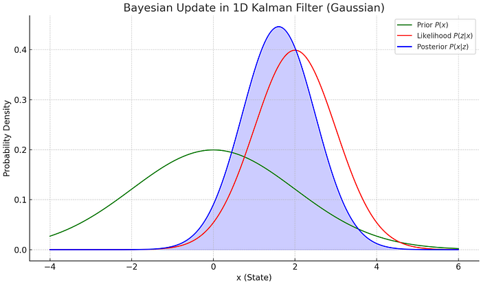
Prior belief P(x): This is the estimate of the state before incorporating the new measurement. It has a certain mean (e.g., from prediction) and variance (uncertainty).
Measurement likelihood P(z∣x): This represents the probability of observing measurement z if the true state were x. It usually has a tighter variance (assuming sensors are precise).
After the measurement and applying Bayes' rule, the Kalman Filter will produce a even tighter new estimate as:
Posterior P(x∣z): The new estimate that combines both sources of information.
- The mean shifts to somewhere between the prior mean and the measurement.
- The variance decreases, because now you have more information (prediction + measurement).
Why the Posterior Is Narrower (more certain)
One of the most powerful aspects of the Kalman Filter is how it reduces uncertainty by combining two sources of information: your prior belief and the measurement.
Kalman filter computes the updated (posterior) variance as:
σ′² = 1 / (1 / r² + 1 / σ²)
Where:
- σ² is the variance of your prior (prediction uncertainty)
- r² is the variance of your measurement (sensor noise)
This formula guarantees:
σ′² < min(r², σ²)
In other words, the updated belief (posterior) is more confident — it has less uncertainty than either the prediction or the measurement alone.
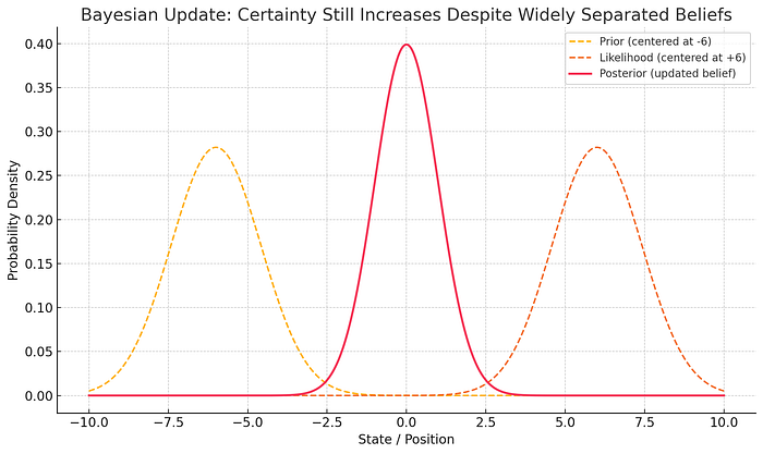
In more extreme case where Prior and Measurement are far apart. Kalman Filter can still produce a more confident estimate, as in the graph below:
The following code demonstrates
- Starts with a very uncertain prior
- Repeatedly: Updates belief using a measurement
- Predicts new state after a motion
You'll see uncertainty (variance) shrink as it gets more confident!
# Measurement update: combine prior estimate with noisy observation
def update_belief(prior_mean, prior_var, meas_value, meas_var):
combined_mean = (meas_var * prior_mean + prior_var * meas_value) / (prior_var + meas_var)
combined_var = 1 / (1 / prior_var + 1 / meas_var)
return [combined_mean, combined_var]
# Prediction step: apply control input or expected motion
def predict_state(current_mean, current_var, motion_change, motion_var):
predicted_mean = current_mean + motion_change
predicted_var = current_var + motion_var
return [predicted_mean, predicted_var]
# Example data
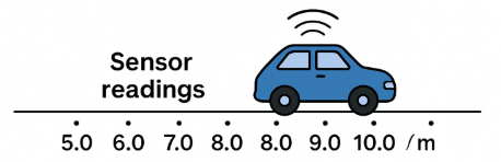
sensor_readings = [5.0, 6.0, 8.0, 9.0] # observed positions
motions_applied = [1.0, 2.0, 2.0, 1.0] # motion per step
sensor_noise = 3.0 # measurement noise (variance)
motion_uncertainty = 2.0 # motion noise (variance)
# Initial guess: very uncertain
estimated_position = 0.0
position_uncertainty = 500.0
# Run Kalman Filter steps
for i in range(len(sensor_readings)):
estimated_position, position_uncertainty = update_belief(
estimated_position, position_uncertainty,
sensor_readings[i], sensor_noise
)
print("Update:", [estimated_position, position_uncertainty])
estimated_position, position_uncertainty = predict_state(
estimated_position, position_uncertainty,
motions_applied[i], motion_uncertainty
)
print("Predict:", [estimated_position, position_uncertainty])
# Final result
print("Final estimate:", [estimated_position, position_uncertainty])2D / multi-D Kalman Filter:
The main difference between 1D and multi-dimensional (2D, 3D, etc.) Kalman Filters lies in the mathematics and data structure used — but the core logic stays the same.
If 1D KF is like Tracks a single scalar variable, like: Position along a line, Temperature, Battery level, 2D / Multi-Dimensional Kalman Filter tracks multiple variables simultaneously, often correlated, like:
- Position (x, y)
- Velocity (vx, vy)
- Acceleration, orientation, etc.
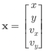
For example, the state vector can be something like:
x = [x_position,
     y_position,
     x_velocity,
     y_velocity]
And the full Kalman Filter algorithm becomes:
✅ The standard symbols used in multi-dimensional Kalman Filters:
- x: state estimate (vector, e.g., position, velocity)
- P: covariance matrix (uncertainty in state)
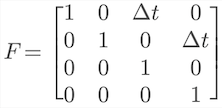
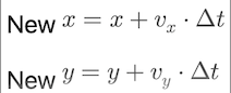
- F: state transition matrix (how state evolves, e.g. for constant velocity motion model and a time step, the F is as below:)
- u: control input (external motion command)
- z: actual sensor measurement
- H: measurement function (how sensor relates to state)
If the measurement doesn't cover all features in the state, for example, state space have 3 element [x, y, z], our sensor can only measure x and y. The H will be
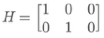
to map from state space [x, y, z] to measurement space [x_m, y_m]
- R: measurement noise covariance
- I: identity matrix (used in update step)
✅ Equations:
Prediction Step:
x' = F * x + u→ predict next state from current state and control inputP' = F * P * Fᵀ→ propagate uncertainty through model
Measurement Update Step:
y = z - H * x→ innovation (difference between actual and expected measurement)S = H * P * Hᵀ + R→ innovation covariance (uncertainty in prediction + measurement)K = P * Hᵀ * S⁻¹→ Kalman gain: how much we trust the measurement vs prediction. It tells us:"Given the uncertainty in my prediction ($P$) and in my sensor ($R$), how much should I shift my prediction toward the measurement?"x' = x + K * y→ update state estimateP' = (I - K * H) * P→ update uncertainty (we've reduced it by using the measurement)
This code snippet demonstrated this method. We get position measurements (noisy), and then Kalman Filter estimates both position and velocity over time and reduces uncertainty.
import numpy as np

# Initial state (position=0, velocity=0)
x = np.array([[0.],    # position
              [0.]])   # velocity
# Initial uncertainty: high uncertainty in velocity
P = np.array([[1000., 0.],
              [0., 1000.]])
# State transition matrix: assumes constant velocity model
dt = 1.0  # time step
F = np.array([[1, dt],
              [0, 1]])
# Control input (optional)
u = np.array([[0.],    # external motion (acceleration influence)
              [0.]])
# Measurement matrix: we can only measure position
H = np.array([[1, 0]])
# Measurement noise covariance (sensor noise)
R = np.array([[1]])
# Identity matrix
I = np.eye(2)
# Measurement sequence (sensor gives positions over time)
measurements = [1, 2, 3]
for z in measurements:
    # --- Prediction Step ---
    x = F @ x + u                        # state prediction
    P = F @ P @ F.T                      # uncertainty prediction
    # --- Measurement Update Step ---
    z = np.array([[z]])                 # convert scalar to vector
    y = z - H @ x                       # innovation
    S = H @ P @ H.T + R                 # innovation covariance
    K = P @ H.T @ np.linalg.inv(S)     # Kalman Gain
    x = x + K @ y                       # updated state
    P = (I - K @ H) @ P                 # updated uncertainty
    print("State estimate:\n", x)
    print("Covariance:\n", P)
    print("-" * 30)
The following plot demonstrates a 2D Kalman Filter estimating both position and velocity over time, with the correlation ellipses visualized at each step:
- Red dots: Estimated (position,velocity) state after each update.
- Blue ellipses: Covariance ellipses showing uncertainty and correlation between position & velocity.
- ρ: Pearson correlation between position and velocity in the covariance matrix.
As the filter progresses:
- The ellipses shrink, meaning uncertainty decreases with more measurements.
- The correlation values ρ stabilize (e.g., ~0.84), showing the increasing confidence in how position and velocity relate.
If you found this useful, follow me for more intuitive robotics explainers — or leave a comment and say hi!
Reference:
Thrun, Sebastian. AI for Robotics.
📘 Also check out my related articles about AI in Robotics: - [Bayes' Rule in Robot Localization] - [SLAM: How Lost Robots Build a Map] - [Kalman Filter — Combining Messy Sensors with Math] - [Particle Filters: An Intuitive Guide to Robot Localization] - [Where AI Robots Take Us, Practically and Philosophically]