All you have is:
- A flashlight (your sensor)
- A notepad (your memory)
Your job is to:
- Figure out where you are (Localization).
- Draw a map (Mapping)
You have to do both at the same time — because you can't localize without a map, and you can't build a map without knowing where you are.
This is SLAM: "Simultaneous Localization and Mapping" .
We're basically trying to solve the classic 🐔🥚 problem: "Which comes first — knowing where you are or building the map?" SLAM says: why not both, together?
Graph SLAM:
One way to solve the SLAM problem is Graph SLAM. It is like a giant puzzle make of constraints.
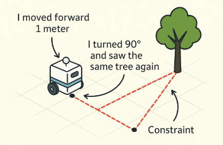
A constraint is just a piece of information about how things relate to each other. For example, it tells us:
" I moved forward 1 meter."
"I turned and saw the same landmark again."
"This position is 5 meters away from that one"
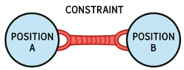
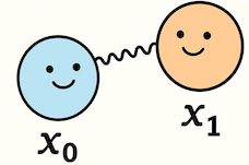
A constraint like a rubber band that pulls two positions toward a certain relationship. It doesn't say exactly where things are — it just says how far apart they should be, or how they're connected.
Overall, in Graph SLAM, the robot is trying to answer:
"Where have I been?"
"Where are the landmarks?"
…based only on the relative movement and noisy sensor data.
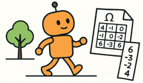
Dive deep into the technical formula:
While the robot is walking around, it collected many clues. Then it put all those clues together and figure out the best guess of:
- Where the robot is at each step (poses).
- Where each landmark is.
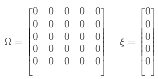
This is where Ω⋅μ = ξ comes in.
Where:
Ω(Omega) is the information matrixμis the vector of unknowns (robot poses, landmarks, etc.)ξ(xi) is the information vector
What Do These Symbols Mean (Intuitively)?
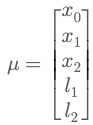
👉 Think of μ as a list of positions:
- Robot at time 0: x₀
- Robot at time 1: x₁
- Robot at time 2: x₂
- Landmark 1: l₁
- Landmark 2: l₂ …and so on.
This is your map + trajectory — the thing you're trying to figure out!
👉Think of Ω (Omega) as how strongly you believe in the clues.
- It's like a giant trust web.
- Each time the robot says "I moved 5m," it ties two positions (say x₀ and x₁) together.
- These become connections in the matrix — like rubber bands with different strengths.
So Omega tells you:
- Which things are connected (via constraints)
- How strong those connections are (based on measurement certainty)
It's called the information matrix because it reflects how much "information" (i.e., certainty) you have.
👉Think of ξ (xi) as all the clues you collected.
- It stores the actual measurements you've made (like "x₁ is 5 meters from x₀").
- It's like your notepad of clues from the world.
👉 In summary Ω⋅μ = ξ can be interpreted as: "How strongly positions are connected" × "The positions themselves" = "What we actually measured."
How do we solve Ω⋅μ = ξ?
The robot builds the matrix (Ω and ξ) as it walks around .…..
Every time the robot moves or makes an observation, it adds a new piece of information — like a clue in a detective notebook.
That clue gets translated into:
- A few numbers added to the matrix Ω (how things are connected)
- And some values added to the vector ξ (actual measurements)
Eventually, it build the Ω and ξ, then we solve the equation to get μ that gives us the best guess of where everything is.
Let's take a look of a real world example:
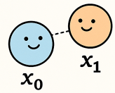
Our robot moves along a hallway and makes two movements:
- It starts at unknown position x0
- x0 → x1 : moves 1 meter forward to x1
- From x1, it sees landmark l1 is 2 meters to the right
- x1 → x2: moves 1 meter forward to x2
- From x2, it sees landmark l2 is 1 meter to the right
We'll estimate the most likely positions for x0,x1,x2,l1, l2 using SLAM.
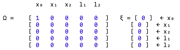
Step 1: Define the Variables
we are solving for:
So we need:
- A 5×5 matrix (Ω)
- A 5×1 vector (ξ)
Step 2: Initialize Ω and ξ with zeros
Step 3: Anchor the first position x_0 = 0
Step 4: Motion constraints
As the robot moves and senses landmarks, it gathers relative measurements. Each constraint is a relative observation. It gaves us a "Rubber Band" between positions.
a ) When:
- x0 → x1 : moves 1 meter forward to x1
x1 — x0 = 1, meaning:
"x₁ is 1 meter ahead of x₀"
This becomes a constraint between two variables (x₀ and x₁). We want to add this info into our system (Ω, ξ) so the final solution for mu = [x0, x1, …] respects this relationship.
We update Ω: Ω[0, 0] += 1 and Ω[1, 1] += 1
This adds weight (trust) to both variables involved.
- You're saying: "I now have one piece of info involving x₀ and one involving x₁."
- So you increase their diagonal values (kind of like boosting their confidence).
Think of it as:
"We know something about x₀ and x₁ now, so let's make their positions matter more."
Next, we update Ω: Ω[0, 1] -= 1 and Ω[1, 0] -= 1
This encodes the relationship between x₀ and x₁.
- It reflects that x₀ and x₁ are not independent — they are tied together.
- The off-diagonal terms form a "rubber band" pulling their values toward each other with a fixed offset of 1.
Think of this as saying:
"The difference between x₀ and x₁ should be 1."
If x₀ goes too far from x₁, this rubber band pulls them back.
Lastly, we update ξ: ξ[0] += -1, ξ[1] += 1
This encodes the actual measurement:
x1 — x0 = 1
Rewriting:
x0 — x1 = -1
- This is where the value of the measurement is stored.
- ξ acts like a "notepad" where the robot writes down what it actually observed.
The updates mean:
"Hey x₀, adjust your belief downward by 1"
"Hey x₁, adjust your belief upward by 1"
Together, this encodes the idea that: x₁ is 1 more than x₀.
🤔You may get confused here that after the update… doesn't the difference between x0 and x1 become 2, instead of 1.
Short Answer: No — it still enforces x1 — x0 = 1.
When building Ω and ξ, we translate it into a least squares problem, which minimizes: (x1 — x0–1)², which is same as (x0 — x1 — (-1))² → x0 — x1 + 1
The vector part (ξ) comes from taking the derivative of this squared error function with respect to x₀ and x₁ — that's where: xi[0] += -1, xi[1] += +1 comes from.
b) Similarly, when:
x1 → x2: moves 1 meter forward to x2
Update:
- Ω[1,1] += 1, Ω[2,2] += 1
- Ω[1,2] -= 1, Ω[2,1] -= 1
- ξ[1] += -1, ξ[2] += 1
Now, we have:
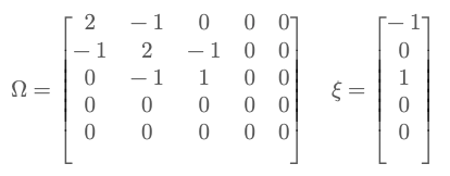
Step 5: Landmark observations
a) From x1, robot sees l1 = x1 + 2
Rewritten as: l1 — x1 = 2
Update:
- Ω[1,1] += 1, Ω[3,3] += 1
- Ω[1,3] -= 1, Ω[3,1] -= 1
- ξ[1] += -2, ξ[3] += 2
b) From x2, robot sees l2 = x2 + 1
Rewritten as: l2 — x2 = 1
Update:
- Ω[2,2] += 1, Ω[4,4] += 1
- Ω[2,4] -= 1, Ω[4,2] -= 1
- ξ[2] += -1, ξ[4] += 1
Now, we finally have:
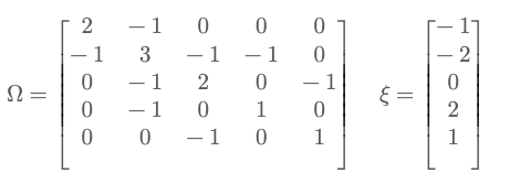
Step 6: Solve Ω⋅μ = ξ
import numpy as np
Omega = np.array([
[2, -1, 0, 0, 0],
[-1, 3, -1, -1, 0],
[0, -1, 2, 0, -1],
[0, -1, 0, 1, 0],
[0, 0, -1, 0, 1]
])
xi = np.array([-1, -2, 0, 2, 1])
mu = np.linalg.solve(Omega, xi)
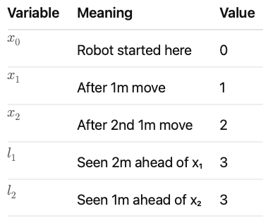
print(mu)Output:
[0. 1. 2. 3. 3.]
Final Interpretation:
📘 Also check out my related articles about AI in Robotics: - [Bayes' Rule in Robot Localization] - [SLAM: How Lost Robots Build a Map] - [Kalman Filter — Combining Messy Sensors with Math] - [Particle Filters: An Intuitive Guide to Robot Localization] - [Where AI Robots Take Us, Practically and Philosophically]