Hands-on Tutorials
Data is the fuel for models, but you may have encountered situations where you also want to incorporate the expert's knowledge into the model, or there is no data available, but solely a domain expert who can describe "the situation" given the circumstances. By reading this blog, you will learn the concepts of knowledge-driven models in terms of Bayesian probabilistic models, and with the hands-on tutorial, you will create a real plan to model an expert's knowledge into a Bayesian model for inferences. Finally, you will learn about the challenges of creating larger and more complex knowledge-driven models so that you can apply them in your own domain. All examples are created using the Python library bnlearn.
If you found this article helpful, you are welcome to follow me because I write more about Bayesian statistics! I recommend experimenting with the hands-on examples in this blog. This will help you to learn quicker, understand better, and remember longer. Grab a coffee and have fun!
A Brief Introduction: The Importance of Human Knowledge.
In today's data-driven world, the emphasis often lies on collecting massive amounts of data and letting machine learning algorithms uncover patterns. While this approach has proven successes in many domains, it also has limitations. The reason is that data alone does not always capture the underlying mechanisms of a system, especially when information is sparse, noisy, biased, or simply unavailable. In such cases, expert knowledge can play a decisive role. The challenge, however, is that human knowledge is often qualitative, ambiguous, or embedded in tacit experience, which makes it difficult for computers to process.
Knowledge-driven models provide a solution by transforming expert insights into computer-interpretable structures. These models allow us to formalize what is already known about a system, combine it with data where available, and reason about outcomes even when observations are limited. This makes them particularly powerful in domains such as healthcare, engineering, policy-making, and risk assessment, where expert judgment has traditionally guided decisions. Unlike purely data-driven approaches, knowledge-driven models enable explanations, causal reasoning, and counterfactual analysis, offering not only predictions but also understanding.
To appreciate the value of knowledge-driven models, it is important to distinguish them from purely statistical associations. Just because two variables appear related in a dataset does not mean one causes the other. Knowledge-driven approaches explicitly encode causal and structural assumptions about the system, reducing the risk of spurious conclusions and improving interpretability. In the following section, we will learn how human knowledge can be seen as a form of data.
Human Knowledge As Data.
When we think of data, we usually imagine numbers in a table or measurements collected from sensors, something concrete, quantitative, and machine-readable. Human knowledge, by contrast, often comes in the form of experience, intuition, or reasoning about how things work. Although this knowledge is also data, it has a place in the human mind rather than in a database. The key idea with knowledge-driven models is that every expert judgment, causal statement, or heuristic rule can be viewed as a piece of information about the world, and therefore as something we can model, quantify, and use computationally.
The first step of treating human knowledge as data is by formalizing what experts know about relationships between variables: which factors influence others? How strong are the relationships? Under what conditions do they occur? For example, a doctor might reason that "a certain symptom usually follows a particular infection". This is not a row in a spreadsheet, but structured observations about dependencies. The same kind of information that statistical models learn from data, only expressed verbally or conceptually.
To make this knowledge useful for machines, we must encode it into a structured representation. We can do this in the form of variables, links, and probabilities. The representation then acts as a bridge between human reasoning and machine computation, transforming qualitative understanding into a quantitative form that can be tested, combined with observed data, and used for inference.
The knowledge being used is as rich as the experts experiences and as colored as the experts prejudices.
By treating human knowledge as data, we unlock the possibility of modeling systems that are partially known or where data is incomplete or too costly to collect. Instead of spending time and effort to create large datasets using sensors and other measurements, we can start from what we already know and refine that knowledge as new information. This is the foundation of knowledge-driven modeling and the stepping stone toward human–machine collaboration in Bayesian modeling.
In the following sections, we will explore how expert knowledge can be captured, represented, and combined with data using Bayesian networks and related methods, and why this approach is increasingly vital in building robust, interpretable, and actionable models.
How To Convert an Expert's Knowledge Into A Model?
There is no doubt that an expert's knowledge is important for so many reasons. The question here is: can we capture, model, and reliably use the information using a model? In general, when we talk about knowledge, it is not solely descriptive knowledge, such as facts. Knowledge is also a familiarity, awareness, or understanding of someone or something, procedural knowledge (skills), or acquaintance knowledge [1]. To capture and model human knowledge, we need to design a system that is built on a sequence of process stages. Or, in other words, a sequence goes from the output of the process into the input of the next process. Multiple simple sequences can then be combined into a complex system.
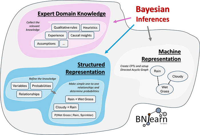
The effectiveness of knowledge-driven modeling lies in two key aspects: representing expert knowledge as a graph structure and unifying it consistently using the principles of probability.
In the figure below, a schematic overview is shown of how human knowledge is captured and structured. The first step (pink) is thus collecting the relevant knowledge in terms of heuristics, rules, experiences, assumptions, and so on. The second step (blue) is to structure this information in terms of variables, relationships, and probabilities. The relationships can be created by simple one-to-one relationships, while determining the probabilities may be more challenging. More about this can be read later in this blog. The last step is to represent the system as a graph with nodes and edges (step 3, gray). Each node corresponds to a variable, and each edge represents conditional dependencies between pairs of variables. In this manner, we can define a model based on the expert's knowledge, and the best way to do that is with Bayesian models.
To build a computer-aided knowledge model, any knowledge you possess or intend to use must be expressed in a form that a computer can interpret.
To answer the question, can we always get experts' knowledge into structured models? The answer is: it depends. One of the crucial parts is how accurately we can represent the knowledge as a graph and how precisely we can glue it together by the probability theorem, a.k.a. Bayesian graphical models. There are various challenges to overcome before we can create a reliable model. Let's jump to the next section, where we will step into the world of Bayesian Graphical models.
How To Use Bayesian Graphical Models For Creating Knowledge-Driven Models?
The use of machine learning techniques has become a standard toolkit to obtain useful insights and make predictions in many domains. However, many of the models are data-driven, which means that data is required to learn a model. Incorporating an expert's knowledge into data-driven models is not possible or straightforward. However, a branch of machine learning is Bayesian graphical models (a.k.a. Bayesian networks, Bayesian belief networks, Bayes Net, causal probabilistic networks, and Influence diagrams), which can be used to incorporate experts' knowledge into models. With such models, we can then make inferences, which is important to describe the probability that a certain state or event occurs. Some of the advantages of Bayesian graphical models are as follows:
- The possibility of incorporating domain/expert knowledge in a graph.
- It has a notion of modularity.
- A complex system is built by combining simpler parts.
- Graph theory provides intuitively highly interacting sets of variables.
- Probability theory provides the glue to combine the parts.
To make Bayesian graphical models, you need two ingredients: 1. Directed Acyclic Graphs (DAG) and 2. Conditional Probabilistic Tables (CPTs). Only if we put them together can it form a representation of the expert's knowledge.
Part 1: Bayesian Graphs are Directed Acyclic Graphs (DAG).
At this point, you know that knowledge can be represented as a systematic process and can be seen as a graph. In the case of Bayesian models, a graph needs to be represented as a DAG. But what exactly is a DAG? First of all, it stands for Directed Acyclic Graphs and is a network (or graph) with nodes (variables) and edges that have one direction (directed). Figure 1 depicts three unique patterns that can be made with three variables (X, Y, Z). Nodes correspond to variables X, Y, Z, and the directed edges (arrows) indicate dependency relationships or conditional distributions. The network is acyclic, which means that no (feedback) loops are allowed.
With a DAG, a complex system can be created by combining the (simpler) parts.
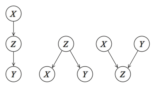
All DAGs (large or small) are built under the following 3 rules:
- Edges are conditional dependencies.
- Edges are directed.
- Feedback loops are not allowed.
These rules are important because if you remove the directionality (or arrows), the three DAGs become identical. Or in other words, with the directionality, we can make the DAG identifiable [2]. Many blogs, articles, and Wikipedia pages describe the statistics and causality behind the DAGs, but what you need to understand is that every Bayesian network can be designed by these three unique patterns. These three patterns are thus representative in every process you want to model. Designing the DAG is the first part of creating a knowledge-driven model. The second part defines the Conditional Probabilistic Tables (CPT); the strength of the relationship at each node in terms of (conditional) probabilities.
Part 2: Define The Conditional Probabilistic Tables To Describe The Strength Of The Node Relationships.
Probability theory (a.k.a. Bayes' theorem or Bayes Rule) forms the foundation for Bayesian networks. Check out this Medium article about Bayesian structure learning [3] for more details:
Although the Bayes theorem is applicable here too, there are some differences. First, in a knowledge-driven model, the CPTs are not learned from data (because there is no data). Instead, the probabilities need to be derived from the expert by questioning and subsequently being stored in so-called Conditional Probabilistic Tables (CPT) (also named Conditional Probability Distribution, CPD). I will use CPT and CPD interchangeably throughout this article.
The CPTs describes the strength of the relationship at each node in terms of conditional probabilities or priors.
The CPTs are then used with the Bayes rule to update model information, which allows making inferences. In the next section, I will demonstrate, with the Sprinkler use case, how to exactly fill in the CPT with expert knowledge. But first, there are challenges in converting experts' knowledge into probabilities.
Converting Expert's Knowledge Into Probabilities.
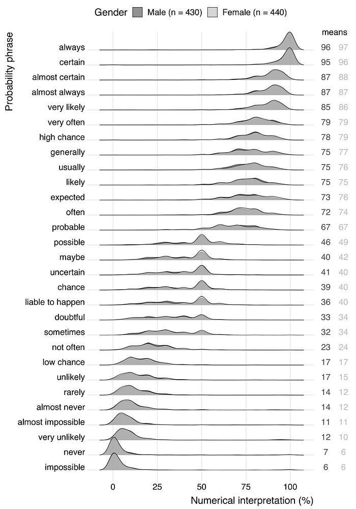
To design a knowledge-driven model, it is crucial to extract the right information from the expert. The domain expert will inform about the probability of a successful process and the risks of side effects. It is super important that the message is understood as intended to minimize the risk of miscommunication. When talking to experts, many estimated probabilities are communicated verbally, with terms such as 'very likely', "sometimes", "always", or "common" instead of exact percentages.
Make sure that the verbal probability phrase is the same for both sender and receiver in terms of probabilities or percentages.
In certain domains, there are guidelines that describe terms. As an example, 'common' can be in the range 30–40%. But without background knowledge of the domain, the word 'common' can easily be interpreted as a different number [4]. In addition, the interpretation of a probability phrase can be influenced by its context [4]. Let's do a small test. For instance, compare your numerical interpretation in the next two statements:
- It will likely rain in Manchester (England) next June.
- It will likely rain in Barcelona (Spain) next June.
Probably, your numerical interpretation of 'likely' in the first statement is higher than in the second. Be cautious of contextual misinterpretations, as they can also lead to systematic errors and thus incorrect models. An overview of probability phrases is shown in Figure 2.
'Impossible' seems not always be impossible!
The BNLearn library for Python.
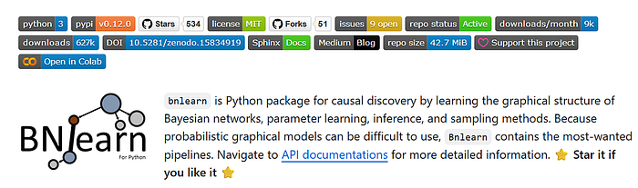
A few words about the bnlearn library that is used for all the analyses in this blog: the bnlearn library provides tools for creating, analyzing, and visualizing Bayesian networks in Python. It supports discrete, mixed, and continuous datasets and is designed to be easy to use while including the most essential Bayesian pipelines for causal learning. With bnlearn, you can perform structure learning, parameter estimation, inference, and create synthetic data, making it suitable for both exploratory analysis and advanced causal discovery. A range of statistical tests can be applied simply by specifying parameters during initialization. Additional helper functions allow you to transform datasets, derive the topological ordering of an entire graph, compare two networks, and generate a wide variety of insightful plots. Core functionalities include:
The key pipelines are:
- Structure Learning: Learn the network structure from data or integrate expert knowledge.
- Parameter Learning: Estimate conditional probability distributions from observed data.
- Inference: Query the network to compute probabilities, simulate interventions, and test causal effects.
- Synthetic Data: Generate new datasets from learned Bayesian networks for simulation, benchmarking, or data augmentation.
- Discretize Data: Transform continuous variables into discrete states using built-in discretization methods for easier modeling and inference.
- Model Evaluation: Compare networks using scoring functions, statistical tests, and performance metrics.
- Visualization: Interactive graph plotting, probability heatmaps, and structure overlays for transparent analysis.
What benefits does bnlearn offer over other Bayesian analysis implementations?
- Contains the most-wanted Bayesian pipelines.
- Simple and intuitive in usage.
- Open-source with MIT Licence.
- Documentation page and blogs.
- +500 stars on GitHub with over 600K downloads.
Use Case: Building A System Based On Experts' Knowledge.
Let's start with a simple and intuitive example to demonstrate the building of a real-world model based on an expert's knowledge.
Suppose you have a sprinkler system in your backyard and, for the last 1000 days, you have witnessed firsthand how and when it works. However, you did not collect any data, but instead you have an intuition about its working. This is what we would call an expert's view or domain knowledge.
As an example, let's assume that from an expert's view, the following propositions about the system are made;
- The Sprinkler system is sometimes on and sometimes off (isn't it great).
- The expert has seen -very often- that if the sprinkler system is on, the grass is Wet.
- However, the expert also knows that rain -almost certainly- results in wet grass and that the sprinkler system is then, most of the time, off.
- The expert also witnessed that the weather was cloudy before it started to rain.
- The expert also noticed a weak interaction between Sprinkler and Cloudy weather, but is not entirely sure about that.
From this point on, you need to convert the expert's propositions into a model. This can be done systematically by first creating the graph based on the interactions and then defining the CPTs that connect the nodes in the graph.
Determine Manually The One-To-One Interactions Based On The Propositions.
A complex system is built by combining simpler parts. This means that you don't need to create or design the whole system at once, but first define the simpler parts. The simpler parts are one-to-one relationships. In this step, we will convert the expert's view into relationships. We know that the Sprinkler system consists of four nodes, each with two states:
- Rain: Yes or No
- Cloudy: Yes or No
- Sprinkler system: On or Off
- Wet grass: True or False
We know from the expert that rain depends on the cloudy state, wet grass depends on the rain state, but wet grass also depends on the sprinkler state. Finally, we know that sprinkler depends on cloudy. We can make the following four directed one-to-one relationships.
- Cloudy → Rain
- Rain → Wet Grass
- Sprinkler → Wet Grass
- Cloudy → Sprinkler
It is important to realize that there are differences in the strength of the relationships between the one-to-one parts that need to be defined using the CPTs. But before stepping into the CPTs, let's first make the DAG using bnlearn.
A DAG Is Based On One-To-One Relationships.
The four directed relationships can now be used to build a graph with nodes and edges. Each node corresponds to a variable, and each edge represents a conditional dependency between pairs of variables. In bnlearn, we can assign and graphically represent the relationships between variables.
# Install the library
pip install bnlearn
# Import library
import bnlearn as bn
# Define the causal dependencies based on your expert/domain knowledge.
# Left is the source, and right is the target node.
edges = [('Cloudy', 'Sprinkler'),
('Cloudy', 'Rain'),
('Sprinkler', 'Wet_Grass'),
('Rain', 'Wet_Grass')]
# Create the DAG
DAG = bn.make_DAG(edges)
# Plot the DAG (static)
bn.plot(DAG)
# Plot the DAG (interactive)
bn.plot(DAG, interactive=True)
# DAG is stored in an adjacency matrix
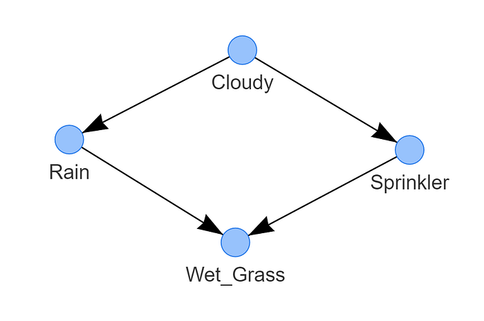
DAG["adjmat"]Figure 3 is the resulting DAG. We call this a causal DAG because we have assumed that the edges we encoded represent our causal assumptions about the sprinkler system.
At this point, the DAG does not know the underlying dependencies. We can check the CPTs with bn.print(DAG)which will result in the message "no CPD can be printed". We need to add knowledge to the DAG with so-called Conditional Probabilistic Tables (CPTs), and we will rely on the expert's knowledge to fill the CPTs.
Knowledge can be added to the DAG with Conditional Probabilistic Tables (CPTs).
Setting up the Conditional Probabilistic Tables.
The sprinkler system is a simple Bayesian network where Wet grass (child node) is influenced by two-parent nodes (Rain and Sprinkler) (see figure 1). The nodes Sprinkler and Rain are influenced by a single node; Cloudy. The Cloudy node is not influenced by any other node.
We need to associate each node with a probability function that takes, as input, a particular set of values for the node's parent variables and gives (as output) the probability of the variable represented by the node. Let's do this for the four nodes.
CPT: Cloudy
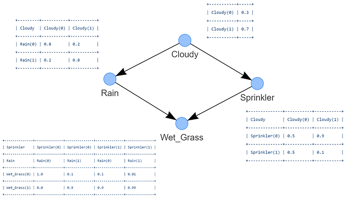
The Cloudy node has two states (yes or no) and no dependencies. Calculating the probability is relatively straightforward when working with a single random variable. From my expert view across the last 1000 days, I have eye-witnessed 70% of the time cloudy weather (I'm not complaining though, just disappointed). As the probabilities should add up to 1, not cloudy should be 30% of the time. The CPT looks as following:
# Import the library
from pgmpy.factors.discrete import TabularCPD

# Cloudy
cpt_cloudy = TabularCPD(variable='Cloudy', variable_card=2, values=[[0.3], [0.7]])
print(cpt_cloudy)
"""
+-----------+-----+
| Cloudy(0) | 0.3 |
+-----------+-----+
| Cloudy(1) | 0.7 |
+-----------+-----+
"""
CPT: Rain
The Rain node has two states and is conditioned by Cloudy, which also has two states. In total, we need to specify 4 conditional probabilities, i.e., the probability of one event given the occurrence of another event. In our case; the probability of the event Rain that occurred given Cloudy. The evidence is thus Cloudy and the variable is Rain. From my expert's view I can tell that when it Rained, it was also Cloudy 80% of the time. I did also see rain 20% of the time without visible clouds (Really? Yes. True story).
# CPT Rain
cpt_rain = TabularCPD(variable='Rain', variable_card=2,
                      values=[[0.8, 0.2],
                              [0.2, 0.8]],
                      evidence=['Cloudy'], evidence_card=[2])
print(cpt_rain)

"""
+---------+-----------+-----------+
| Cloudy  | Cloudy(0) | Cloudy(1) |
+---------+-----------+-----------+
| Rain(0) | 0.8       | 0.2       |
+---------+-----------+-----------+
| Rain(1) | 0.2       | 0.8       |
+---------+-----------+-----------+
"""
CPT: Sprinkler
The Sprinkler node has two states and is conditioned by the two states of Cloudy. In total, we need to specify 4 conditional probabilities. Here we need to define the probability of Sprinkler given the occurrence of Cloudy. The evidence is thus Cloudy and the variable is Rain. I can tell that when the Sprinkler was off, it was Cloudy 90% of the time. The counterpart is thus 10% for Sprinkler is true and Cloudy is true. Other probabilities I'm not sure about, so I will set it to 50% of the time.
cpt_sprinkler = TabularCPD(variable='Sprinkler', variable_card=2,
                           values=[[0.5, 0.9],
                                   [0.5, 0.1]],
                           evidence=['Cloudy'], evidence_card=[2])
print(cpt_sprinkler)

"""
+--------------+-----------+-----------+
| Cloudy       | Cloudy(0) | Cloudy(1) |
+--------------+-----------+-----------+
| Sprinkler(0) | 0.5       | 0.9       |
+--------------+-----------+-----------+
| Sprinkler(1) | 0.5       | 0.1       |
+--------------+-----------+-----------+
"""
CPT: Wet grass
The wet grass node has two states and is conditioned by two-parent nodes; Rain and Sprinkler. Here we need to define the probability of wet grass given the occurrence of rain and sprinkler. In total, we have to specify 8 conditional probabilities (2 states ^ 3 nodes).
- As an expert, I am certain, let's say 99%, about seeing wet grass after raining or sprinkler was on:
P(wet grass=1 | rain=1, sprinkler =1) = 0.99. The counterpart is thusP(wet grass=0| rain=1, sprinkler =1) = 1–0.99 = 0.01 - As an expert, I am entirely sure about no wet grass when it did not rain or the sprinkler was not on:
P(wet grass=0 | rain=0, sprinkler =0) = 1. The counterpart is thus:P(wet grass=1 | rain=0, sprinkler =0) = 1–1= 0 - As an expert, I know that wet grass almost always occurred when it was raining and the sprinkler was off (90%).
P(wet grass=1 | rain=1, sprinkler=0) = 0.9. The counterpart is:P(wet grass=0 | rain=1, sprinkler=0) = 1–0.9 = 0.1. - As an expert, I know that Wet grass almost always occurred when it was not raining and the sprinkler was on (90%).
P(wet grass=1 | rain=0, sprinkler =1) = 0.9. The counterpart is:P(wet grass=0 | rain=0, sprinkler =1) = 1–0.9 = 0.1.
cpt_wet_grass = TabularCPD(variable='Wet_Grass', variable_card=2,
                           values=[[1, 0.1, 0.1, 0.01],
                                   [0, 0.9, 0.9, 0.99]],
                           evidence=['Sprinkler', 'Rain'],
                           evidence_card=[2, 2])
print(cpt_wet_grass)

"""
+--------------+--------------+--------------+--------------+--------------+
| Sprinkler    | Sprinkler(0) | Sprinkler(0) | Sprinkler(1) | Sprinkler(1) |
+--------------+--------------+--------------+--------------+--------------+
| Rain         | Rain(0)      | Rain(1)      | Rain(0)      | Rain(1)      |
+--------------+--------------+--------------+--------------+--------------+
| Wet_Grass(0) | 1.0          | 0.1          | 0.1          | 0.01         |
+--------------+--------------+--------------+--------------+--------------+
| Wet_Grass(1) | 0.0          | 0.9          | 0.9          | 0.99         |
+--------------+--------------+--------------+--------------+--------------+
"""
This is it! At this point, we defined the strength of the relationships in the DAG with the CPTs. Now we need to connect the DAG with the CPTs.
Update the DAG with CPTs:
All the CPTs are created, and we can now connect them with the DAG. As a sanity check, the CPTs can be examined using the print_DAG functionality.
# Update DAG with the CPTs
model = bn.make_DAG(DAG, CPD=[cpt_cloudy, cpt_sprinkler, cpt_rain, cpt_wet_grass])

# Print the CPTs
bn.print_CPD(model)


"""
[bnlearn] >Update current DAG with custom CPD.
[bnlearn] >bayes DAG created.
[bnlearn] >[CPD > Update  ] >[Node Cloudy]
[bnlearn] >[CPD > Update  ] >[Node Sprinkler]
[bnlearn] >[CPD > Update  ] >[Node Rain]
[bnlearn] >[CPD > Update  ] >[Node Wet_Grass]
[bnlearn] >[CPD > Validate] >[Node Cloudy] >OK
[bnlearn] >[CPD > Validate] >[Node Sprinkler] >OK
[bnlearn] >[CPD > Validate] >[Node Rain] >OK
[bnlearn] >[CPD > Validate] >[Node Wet_Grass] >OK

[bnlearn] >[CPD] >[Node Cloudy]:
+-----------+-----+
| Cloudy(0) | 0.3 |
+-----------+-----+
| Cloudy(1) | 0.7 |
+-----------+-----+

[bnlearn] >[CPD] >[Node Sprinkler]:
+--------------+-----------+-----------+
| Cloudy       | Cloudy(0) | Cloudy(1) |
+--------------+-----------+-----------+
| Sprinkler(0) | 0.5       | 0.9       |
+--------------+-----------+-----------+
| Sprinkler(1) | 0.5       | 0.1       |
+--------------+-----------+-----------+

[bnlearn] >[CPD] >[Node Rain]:
+---------+-----------+-----------+
| Cloudy  | Cloudy(0) | Cloudy(1) |
+---------+-----------+-----------+
| Rain(0) | 0.8       | 0.2       |
+---------+-----------+-----------+
| Rain(1) | 0.2       | 0.8       |
+---------+-----------+-----------+

[bnlearn] >[CPD] >[Node Wet_Grass]:
+--------------+--------------+--------------+--------------+--------------+
| Sprinkler    | Sprinkler(0) | Sprinkler(0) | Sprinkler(1) | Sprinkler(1) |
+--------------+--------------+--------------+--------------+--------------+
| Rain         | Rain(0)      | Rain(1)      | Rain(0)      | Rain(1)      |
+--------------+--------------+--------------+--------------+--------------+
| Wet_Grass(0) | 1.0          | 0.1          | 0.1          | 0.01         |
+--------------+--------------+--------------+--------------+--------------+
| Wet_Grass(1) | 0.0          | 0.9          | 0.9          | 0.99         |
+--------------+--------------+--------------+--------------+--------------+

[bnlearn] >Independencies:
(Wet_Grass ⟂ Cloudy | Sprinkler, Rain)
(Sprinkler ⟂ Rain | Cloudy)
(Cloudy ⟂ Wet_Grass | Sprinkler, Rain)
(Rain ⟂ Sprinkler | Cloudy)
[bnlearn] >Nodes: ['Cloudy', 'Sprinkler', 'Rain', 'Wet_Grass']
[bnlearn] >Edges: [('Cloudy', 'Sprinkler'), ('Cloudy', 'Rain'), ('Sprinkler', 'Wet_Grass'), ('Rain', 'Wet_Grass')]
"""
The DAG with CPTs will now be like Figure 4.
Make inferences on the causal model.
Nice work! At this point, you created a model that describes the structure of the data, and the CPTs that quantitatively describe the statistical relationship between each node and its parents. Let's ask some questions to our model and make inferences!
How probable is having wet grass given the sprinkler is off?
q1 = bn.inference.fit(model, variables=['Wet_Grass'], evidence={'Sprinkler': 0})

"""
+----+-------------+----------+
|    |   Wet_Grass |        p |
+====+=============+==========+
|  0 |           0 | 0.383846 |
+----+-------------+----------+
|  1 |           1 | 0.616154 |
+----+-------------+----------+

Summary for variables: ['Wet_Grass']
Given evidence: Sprinkler=0

Wet_Grass outcomes:
- Wet_Grass: 0 (38.4%)
- Wet_Grass: 1 (61.6%)
"""
How probable is a rainy day given sprinkler is off and it is cloudy?
q2 = bn.inference.fit(model, variables=['Rain'], evidence={'Sprinkler':0, 'Cloudy':1})

"""
+----+--------+-----+
|    |   Rain |   p |
+====+========+=====+
|  0 |      0 | 0.2 |
+----+--------+-----+
|  1 |      1 | 0.8 |
+----+--------+-----+

Summary for variables: ['Rain']
Given evidence: Sprinkler=0, Cloudy=1

Rain outcomes:
- Rain: 0 (20.0%)
- Rain: 1 (80.0%)

P(Rain=1 | Sprinkler=0, Cloudy=1) = 0.8
"""
Inferences with two or more variables can also be made, such as:
What are the probabilities for the states Wet grass, Rain given is Sprinkler is On?
q3 = bn.inference.fit(model, variables=['Wet_Grass','Rain'], evidence={'Sprinkler':1})

"""
+----+-------------+--------+------------+
|    |   Wet_Grass |   Rain |          p |
+====+=============+========+============+
|  0 |           0 |      0 | 0.0609091  |
+----+-------------+--------+------------+
|  1 |           0 |      1 | 0.00390909 |
+----+-------------+--------+------------+
|  2 |           1 |      0 | 0.548182   |
+----+-------------+--------+------------+
|  3 |           1 |      1 | 0.387      |
+----+-------------+--------+------------+

Summary for variables: ['Wet_Grass', 'Rain']
Given evidence: Sprinkler=1

Wet_Grass outcomes:
- Wet_Grass: 0 (6.5%)
- Wet_Grass: 1 (93.5%)

Rain outcomes:
- Rain: 0 (60.9%)
- Rain: 1 (39.1%)
"""
How Do I Know My Causal Model Is Right?
In the sprinkler example, we extracted the domain expert's knowledge by making propositions. We created a causal diagram, but when complexity increases, it can become troublesome to verify the validity and completeness of the causal diagram. For example, you may have a different perspective on the probabilities and the graph, and you may also be right about that. As an example, the proposition was given: rain was seen in 20% of the time without visible clouds. It may be reasonable to argue about such a statement. On the contrary, it can also occur that multiple true knowledge models can exist at the same time. In such a case, you may need to combine the probabilities or figure out who is right. Or, in other words, the probabilities we extract by questioning an expert are subjective probabilities [5]. In the sprinkler example, it is sufficient to accept that this notion of probability is personal; it reflects the degree of belief of a particular person at a particular location at a particular time. Question yourself this: will the Sprinkler model change if the expert lives in England compared to Spain?
If you want to use such a procedure to design a knowledge-driven model, it is important to understand how people (experts) arrive at probabilistic estimations. In literature, it is described that people rarely follow the principles of probability when reasoning about uncertain events; rather, they replace the laws of probability with a limited number of heuristics [6, 7], such as representativeness, availability, and adjustment from an anchor. Note that this can lead to systematic errors and, to that extent, incorrect models. Also, make sure that the verbal probability phrase is the same for both sender and receiver in terms of exact probabilities or percentages.
Complexity Is A Major Limitation In Real Use Cases.
The presented sprinkler system has only a few nodes, and therefore is practical for explanation purposes. However, when working with real use-cases, Bayesian networks can contain many more nodes with multiple levels of parent-child dependencies. The number of probability distributions required to populate a conditional probability table (CPT) in a Bayesian network grows exponentially with the number of parent nodes associated with that table. This basically means that if a node has many input relationships, the probability table becomes very complicated and a considerable cognitive barrier [8].
Too much levels of parent-child dependencies can form a considerable cognitive barrier for the domain expert.
For example, if m parent nodes represent Boolean variables, then the probability function is represented by a table of 2^m entries, one entry for each of the possible parent combinations. Be hesitant about creating large graphs (more than 10–15 nodes) as the number of parent-child dependencies can form a considerable cognitive barrier for the domain expert. If you have data for the system that you want to model, it is also possible to learn the structure (DAG), and/or its parameters (CPTs) using structure learning [3].
Beyond The Basics: Generate Synthetic Data From the Human Models.
The designed model, based on the expert's knowledge, can now also be used to generate categorical synthetic data that mimics expert knowledge. The aim in this section is to generate synthetic data that closely mirrors the expert knowledge. In order to do this, we must have a working Bayesian model system that can then be used to generate data and should mimic the knowledge of the expert.
For this use part, we will start without a dataset and define the DAG and CPTs ourselves for a more realistic and complex predictive maintenance use case. Suppose that we need to understand how Machine failures occur, but there are no physical sensors that measure data. An expert can provide us with the following information about the operational activities:
Machine failures are mainly seen when the process temperature is high or the torque is high. A high torque or tool wear causes overstrain failures (OSF). The proces temperature is influenced by the air temperature.
Define simple one-to-one relationships.
From this point on, we need to convert the expert's knowledge into a Bayesian model. This can be done systematically by first creating the graph and then defining the CPTs that connect the nodes in the graph.
A complex system is built by combining simpler parts. This means that we don't need to create or design the whole system at once, but we can define the simpler parts first. These are the one-to-one relationships. In this step, we will convert the expert's view into relationships. We know from the expert that we can make the following directed one-to-one relationships:
Process Temperature→Machine FailureTorque→Machine FailureTorque→Overstrain Failure (OSF)Tool Wear→Overstrain Failure (OSF)Air Temperature→Process TemperatureOverstrain Failure (OSF)→Machine Failure
A DAG is based on one-to-one relationships.
The directed relationships can now be used to build a graph with nodes and edges. Each node corresponds to a variable, and each edge represents a conditional dependency between pairs of variables. In bnlearn, we can assign and graphically represent the relationships between variables.
import bnlearn as bn

# Define the causal dependencies based on your expert/domain knowledge.
# Left is the source, and right is the target node.
edges = [('Process Temperature', 'Machine Failure'),
         ('Torque', 'Machine Failure'),
         ('Torque', 'Overstrain Failure (OSF)'),
         ('Tool Wear', 'Overstrain Failure (OSF)'),
         ('Air Temperature', 'Process Temperature'),
         ('Overstrain Failure (OSF)', 'Machine Failure'),
         ]

# Create the DAG
DAG = bn.make_DAG(edges)

# DAG is stored in an adjacency matrix
DAG["adjmat"]

# Plot the DAG (static)
bn.plot(DAG)

# Plot the DAG
dotgraph = bn.plot_graphviz(DAG, edge_labels='pvalue')
dotgraph.view(filename='bnlearn_predictive_maintanance_expert.pdf')
The resulting DAG is shown in the figure below. We call this a causal DAG because we have assumed that the edges we encoded represent our causal assumptions about the predictive maintenance system.
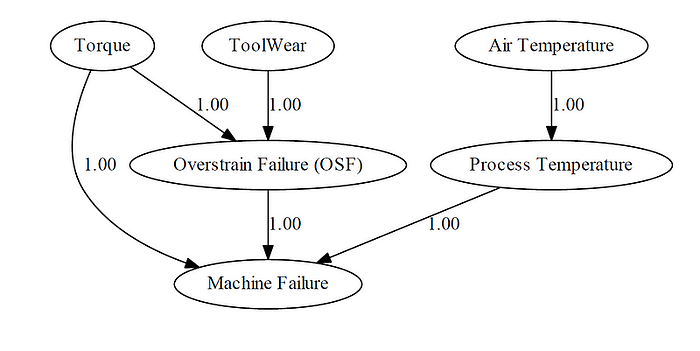
At this point, the DAG does not know the underlying dependencies. Or in other words, there are no differences in the strength of the relationships between the one-to-one parts, but these need to be defined using the CPTs. We can check the CPTs with bn.print(DAG) which will result in the message that no CPD can be printed. We need to add knowledge to the DAG with so-called Conditional Probabilistic Tables (CPTs) and we will rely on the expert's knowledge to fill the CPTs.
Knowledge can be added to the DAG with Conditional Probabilistic Tables (CPTs).
Setting up the Conditional Probabilistic Tables.
The predictive maintenance system is a simple Bayesian network where the child nodes are influenced by the parent nodes. We now need to associate each node with a probability function that takes, as input, a particular set of values for the node's parent variables and gives (as output) the probability of the variable represented by the node. Let's do this for the six nodes.
CPT: Air Temperature
The Air Temperature node has two states: low and high, and no parent dependencies. This means we can directly define the prior distribution based on expert assumptions or historical distributions. Suppose that 70% of the time, machines operate under low air temperature and 30% under high.
- CPT: Tool Wear: Represents whether the tool is still in a low wear or high wear state. It also has no parent dependencies, so its distribution is directly specified. Based on domain knowledge, let's assume 80% of the time, the tools are in low wear, and 20% of the time in high wear.
- CPT: Torque: Torque is a root node as well, with no dependencies. It reflects the rotational force in the process. Let's assume high torque is relatively rare, occurring only 10% of the time, with 90% of processes running at normal torque.
- CPT: Process Temperature: Process Temperature depends on Air Temperature. Higher air temperatures generally lead to higher process temperatures, although there's some variability. The probabilities reflect the following assumptions:
IfAir Tempis low → 70% chance of lowProcess Temp, 30% highandIfAir Tempis high → 20% low, 80% high. - CPT: Overstrain Failure (OSF): Overstrain Failure (OSF) occurs when either Torque or Tool Wear are high. If both are high, the risk increases. The CPT is structured to reflect:
Low Torque & Low Tool Wear → 10% OSFandHigh Torque & High Tool Wear → 90% OSFandMixed combinations → 30–50% OSF. - PT: Machine Failure: The Machine Failure node is the most complicated one because it has the most dependencies: Process Temperature, Torque, and Overstrain Failure (OSF). The risk of failure increases if Process Temp is high, Torque is high, and an OSF occurred. The CPT reflects the additive risk, assigning the highest failure probability when all three are problematic:
Update the DAG with CPTs:
This is it! At this point, we defined the strength of the relationships in the DAG with the CPTs. Now we need to connect the DAG with the CPTs. As a sanity check, the CPTs can be examined using the bn.print_CPD() functionality.
from pgmpy.factors.discrete import TabularCPD

# Air Temperature
cpt_air_temp = TabularCPD(variable='Air Temperature', variable_card=2,
                          values=[[0.7],    # P(Air Temperature = Low)
                                  [0.3]])   # P(Air Temperature = High)

# Tool Wear
cpt_toolwear = TabularCPD(variable='Tool Wear', variable_card=2,
                          values=[[0.8],    # P(Tool Wear = Low)
                                  [0.2]])   # P(Tool Wear = High)

# Torque
cpt_torque = TabularCPD(variable='Torque', variable_card=2,
                        values=[[0.9],     # P(Torque = Normal)
                                [0.1]])    # P(Torque = High)

# Process Temperature
cpt_process_temp = TabularCPD(variable='Process Temperature', variable_card=2,
                               values=[[0.7, 0.2],     # P(ProcTemp = Low | AirTemp = Low/High)
                                       [0.3, 0.8]],    # P(ProcTemp = High | AirTemp = Low/High)
                               evidence=['Air Temperature'],
                               evidence_card=[2])

# Overstrain Failure (OSF)
cpt_osf = TabularCPD(variable='Overstrain Failure (OSF)', variable_card=2,
                     values=[[0.9, 0.5, 0.7, 0.1],  # OSF = No | Torque, Tool Wear
                             [0.1, 0.5, 0.3, 0.9]], # OSF = Yes | Torque, Tool Wear
                     evidence=['Torque', 'Tool Wear'],
                     evidence_card=[2, 2])

# Machine Failure
cpt_machine_fail = TabularCPD(variable='Machine Failure', variable_card=2,
                               values=[[0.9, 0.7, 0.6, 0.3, 0.8, 0.5, 0.4, 0.2],  # Failure = No
                                       [0.1, 0.3, 0.4, 0.7, 0.2, 0.5, 0.6, 0.8]], # Failure = Yes
                               evidence=['Process Temperature', 'Torque', 'Overstrain Failure (OSF)'],
                               evidence_card=[2, 2, 2])


# Update DAG with the CPTs
model = bn.make_DAG(DAG, CPD=[cpt_process_temp, cpt_machine_fail, cpt_torque, cpt_osf, cpt_toolwear, cpt_air_temp])

# Print the CPDs (Conditional Probability Distributions)
bn.print_CPD(model)
Generate Synthetic Data.
At this point, we have our manually defined DAG, and we have estimated the parameters for the CPTs. This means that we captured the system in a probabilistic graphical model, which can now be used to generate synthetic data. We can now use the bn.sampling() function (see the code block below) and generate, for example, 100 samples. The output is a full dataset with all dependent variables.
# Generate synthetic data with 1000 new data points

X = bn.sampling(model, n=1000, methodtype='bayes')

print(X)
+---------------------+------------------+--------+----------------------------+----------+---------------------+
| Process Temperature | Machine Failure  | Torque | Overstrain Failure (OSF)   | ToolWear | Air Temperature     |
+---------------------+------------------+--------+----------------------------+----------+---------------------+
|         1           |        0         |   1    |             0              |    0     |         1           |
|         0           |        0         |   1    |             1              |    1     |         1           |
|         1           |        0         |   1    |             0              |    0     |         1           |
|         1           |        1         |   1    |             1              |    1     |         1           |
|         0           |        0         |   0    |             0              |    0     |         0           |
|        ...          |       ...        |  ...   |            ...             |   ...    |        ...          |
|         0           |        0         |   1    |             1              |    1     |         0           |
|         1           |        1         |   1    |             1              |    1     |         0           |
|         0           |        0         |   0    |             0              |    1     |         0           |
|         1           |        1         |   1    |             1              |    1     |         0           |
|         1           |        0         |   0    |             0              |    1     |         0           |
+---------------------+------------------+--------+----------------------------+----------+---------------------+
If you want more details about data generation, I recommend reading this blog:
Final Words
An advantage of Bayesian networks is that it is intuitively easier for a human to understand direct dependencies and local distributions than complete joint distributions. To make knowledge-driven models, we need two ingredients: the DAG and Conditional Probabilistic Tables (CPTs). Both are derived from the expert through questioning. The DAG describes the structure of the data, and CPTs are needed to quantitatively describe the statistical relationship between each node and its parents. Although such an approach seems reasonable, you should be aware of systematic errors that can occur by questioning the expert, and the limitations when building a complex model.
This is it. Creating a knowledge-driven model is challanging. It is not only about data modeling but also about human psychology. Make sure you prepare for the expert interviews. It is better to have multiple short interviews than one long interview. Ask your questions systematically. First, design the graph with nodes and edges, then go into the CPTs. Be cautious when discussing probabilities. Understand how the expert derives his probabilities and normalize when required. Check if time and place can differ in the outcome. Make sanity checks after building the model. Smile occasionally.
Be Safe. Stay Frosty.
Cheers, E.
I hope you enjoyed reading this article! You are welcome to follow me because I write more about Bayesian statistics! I recommend experimenting with the hands-on examples in this blog. This will help you to learn quicker, understand better, and remember longer. Grab a coffee and have fun!
Software
Let's connect!
References
- Wikipedia, Knowledge
- Pearl, Judea (2000). Causality: Models, Reasoning, and Inference. Cambridge University Press. ISBN 978–0–521–77362–1. OCLC 42291253.
- E. Taskesen, The Starters Guide to Causal Structure Learning with Bayesian Methods in Python, Data Science Collective (DSC), September 2025
- Sanne Willems, et al, Variability in the interpretation of probability phrases used in Dutch news articles — a risk for miscommunication, JCOM, 24 March 2020
- R. Jeffrey, Subjective Probability: The Real Thing, Cambridge University Press, Cambridge, UK, 2004.
- A. Tversky and D. Kahneman, Judgment under Uncertainty: Heuristics and Biases, Science, 1974
- Tversky, and D. Kahneman, 'Judgment under uncertainty: Heuristics and biases,' in Judgment under Uncertainty: Heuristics and Biases, D. Kahneman, P. Slovic, and A. Tversky, eds., Cambridge University Press, Cambridge, 1982, pp 3–2
- Balaram Das, Generating Conditional Probabilities for Bayesian Networks: Easing the Knowledge Acquisition Problem. Arxiv
- E. Taskesen, Synthetic Data: The Essentials Of Data Generation Using Bayesian Sampling., Data Science Collective (DSC), May 2025
- E. Taskesen, Why Prediction Isn't Enough: Using Bayesian Models to Change the Outcome., Data Science Collective (DSC), June 2025