Six Causal Libraries Compared: Which Bayesian Approach Finds Hidden Causes in Your Data?

Deep-dive

Understanding the causal effect of variables in systems or processes is important. However, it can be challenging to get started with Bayesian models, as there are multiple libraries with their own strengths and weaknesses. In this blog, we will compare six popular causal inference libraries in their functionality, ease of use, and flexibility. All libraries are compared using hands-on examples for the same data set and in the same context. The included libraries are Bnlearn, Pgmpy, CausalNex, DoWhy, Pyagrum, and CausalImpact. By the end of this blog, you will have a better understanding of these six causal inference libraries, and allow you to select the causal library that best fits your use case.

If you found this article helpful, you are welcome to follow me because I write more about data science! I recommend experimenting with the hands-on examples in this blog. This will help you to learn quicker, understand better, and remember longer. Grab a coffee and have fun! Disclaimer: I am the author of the BNlearn Library for Python, but I've kept these comparisons objective and unbiased.

A Brief Introduction to Bayesian Modeling.

Causal inference is the process of determining the cause-and-effect relationships between variables in a process or system. In general, we can separate variables into two distinct groups: driver and passenger variables. Driver variables are those that directly influence the outcome or dependent variable, while passenger variables are those that do not have a direct effect but are correlated/ associated with the outcome variable.

The identification of driver variables can be crucial in projects such as predictive maintenance or in the security domain. The driver variables can help explain the causal relationship between the predictor and outcome variables. In contradiction, passenger variables do not have a direct effect on the outcome variable. However, they can still be useful as they can provide additional variation and thus an understanding of the context in which the data was collected.

For example, if we find that engine failures are strongly correlated with location, we might suspect that there is an underlying driver variable that is causing the failure for a specific location.

Causal inference helps to make better decisions by identifying which variables to manipulate and which variables to monitor. More details about Bayesian modeling can be found in this blog.

In causal inference, we move beyond prediction to identify the mechanisms and pathways through which events arise.

Overall, performing causal inference analysis is challenging because it requires separating the effects of multiple variables, accounting for confounding variables, and dealing with uncertainty. Luckily, Python has several libraries that can help data scientists perform causal inference. In this article, we will go through six of the most popular causal inference libraries in Python: Bnlearn, Pgmpy, DoWhy, CausalNex, Pyagrum, and CausalImpact.

Six Popular Causal Inference Libraries For Python.

To evaluate the strengths and limitations of different Bayesian libraries, we will examine six popular packages side by side. For consistency, the same dataset will be used across all libraries whenever possible: the Census Income dataset. This multivariate dataset contains 48,842 instances across 14 variables, each with multiple discrete states. A central question we will explore is whether holding a graduate degree increases the likelihood of earning more than $50K annually. In the code block below, we load and prepare the dataset, which is then used for all analyses.

# Installation
pip install datazets
# Import library
import datazets as dz
import pandas as pd
import numpy as np
import matplotlib.pyplot as plt

# Import data set and drop continous and sensitive features
df = dz.import_example(data='census_income')

# Data cleaning
drop_cols = ['age', 'fnlwgt', 'education-num', 'capital-gain', 'capital-loss', 'hours-per-week', 'race', 'sex']
df.drop(labels=drop_cols, axis=1, inplace=True)

# Print
df.head()

#          workclass  education  ... native-country salary
#0         State-gov  Bachelors  ...  United-States  <=50K
#1  Self-emp-not-inc  Bachelors  ...  United-States  <=50K
#2           Private    HS-grad  ...  United-States  <=50K
#3           Private       11th  ...  United-States  <=50K
#4           Private  Bachelors  ...           Cuba  <=50K
#
#[5 rows x 7 columns]

1. Bnlearn For Python.

The bnlearn library provides tools for creating, analyzing, and visualizing Bayesian networks in Python. It supports discrete, mixed, and continuous datasets and is designed to be easy to use while including the most essential Bayesian pipelines for causal learning. With bnlearn, you can perform structure learning, parameter estimation, inference, and create synthetic data, making it suitable for both exploratory analysis and advanced causal discovery. A range of statistical tests can be applied simply by specifying parameters during initialization. Additional helper functions allow you to transform datasets, derive the topological ordering of an entire graph, compare two networks, and generate a wide variety of insightful plots. Core functionalities include:

• Structure Learning: Learn the network structure from data or integrate expert knowledge.
• Parameter Learning: Estimate conditional probability distributions from observed data.
• Inference: Query the network to compute probabilities, simulate interventions, and test causal effects.
• Synthetic Data: Generate new datasets from learned Bayesian networks for simulation, benchmarking, or data augmentation.
• Discretize Data: Transform continuous variables into discrete states using built-in discretization methods for easier modeling and inference.
• Model Evaluation: Compare networks using scoring functions, statistical tests, and performance metrics.
• Visualization: Interactive graph plotting, probability heatmaps, and structure overlays for transparent analysis.

Bayesian networks built with bnlearn can be used for various tasks, among others, to uncover hidden relationships, test causal hypotheses, and generate synthetic data. More details about inferences and generating synthetic data can be found here:

One of the great functionalities of Bnlearn for Python is that it can learn the causal structure in an unsupervised manner. This means that you do not need to specify any target variable because it will figure it out by itself. There are various search and scoring strategies implemented for this task:

• Search strategies: Hillclimbsearch, Exhaustivesearch, Constraint search, Chow-liu, Naive bayes, and TAN
• Scoring strategies: BIC, K2, BDEU.

Some strategies require setting a root node, such as Tree-augmented Naive Bayes (TAN), which are recommended in case you know the outcome (or target) value. This will also dramatically lower the computational burden and is recommended in case you have many features. In addition, with the independence test, spurious edges can be easily pruned from the model. In the following example, I will use the hillclimbsearch method with scoring type BIC for structure learning. In this example, we will not define a target value but let the Bnlearn decide the entire causal structure purely on the data itself.

# Installation
pip install bnlearn
# Load library
import bnlearn as bn

# Structure learning
model = bn.structure_learning.fit(df, methodtype='hillclimbsearch', scoretype='bic')

# Test edges significance and remove.
model = bn.independence_test(model, df, test="chi_square", alpha=0.05, prune=True)

# Learn the parameters (optional)
model = bn.parameter_learning.fit(model, df)

# Make plot
G = bn.plot(model, interactive=False)

# Ceate dotgraph plot
dotgraph = bn.plot_graphviz(model)
dotgraph.view(filename=r'c:/temp/bnlearn_plot')

# Make plot interactive
G = bn.plot(model, interactive=True)

# Show edges
print(model['model_edges'])
"""
[('education', 'occupation'),
 ('marital-status', 'relationship'),
 ('occupation', 'workclass'),
 ('relationship', 'salary'),
 ('relationship', 'education'),
 ('salary', 'education')]
"""

To determine the Directed Acyclic Graph (DAG), we need to specify the input data frame as shown in the code section above. After fitting a model, the results are stored in the model dictionary, which can be used for further analysis. Both the static plot and interactive plot of the causal structure are shown below.

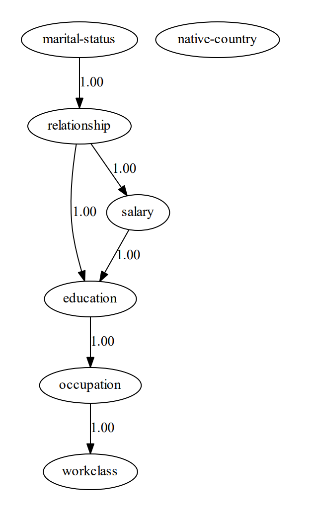
With the learned DAG (Figure 1), we can estimate the conditional probability distributions (CPDs, see code section below), and make inferences using do-calculus. Or in other words, we can start asking questions to our data.

# Learn the CPDs using the estimated edges.
# Note that we can also customize the edges or manually provide a DAG.
# model = bn.make_DAG(model['model_edges'])

# Learn the CPD by providing the model and dataframe
model = bn.parameter_learning.fit(model, df)

# Print the CPD
CPD = bn.print_CPD(model)

Question 1: What is the probability of having a salary > 50k given the education is Doctorate:

P(salary | education=Doctorate)

Intuitively, we may expect a high probability because the education is doctorate. Let's find out the posterior probability from our Bayesian model. In the code section below, we derived a probability of P=0.7093. This confirms that when education is doctorate, there is a higher probability of having a salary of >50K compared to not having a doctorate education.

# Start making inferences
query = bn.inference.fit(model, variables=['salary'], evidence={'education':'Doctorate'})
print(query)

"""
+---------------+---------------+
| salary        |   phi(salary) |
+===============+===============+
| salary(<=50K) |        0.2907 |
+---------------+---------------+
| salary(>50K)  |        0.7093 |
+---------------+---------------+

Summary for variables: ['salary']
Given evidence: education=Doctorate

salary outcomes:
- salary: <=50K (29.1%)
- salary: >50K (70.9%)
"""

Let's now ask the question of whether lower education also results in a lower probability of having a salary of >50K. We can easily change education in HS-grad and again ask the question.

Question 2: What is the probability of having a salary > 50k given the education is HS-grad:

P(salary | education=HS-grad)

This results in a posterior probability of P=0.1615 . Studying is thus very beneficial for a higher salary, according to this data set. However, be aware that we did not use any other constraints as evidence that can influence the outcome.

query = bn.inference.fit(model, variables=['salary'], evidence={'education':'HS-grad'})
print(query)

"""
+---------------+---------------+
| salary        |   phi(salary) |
+===============+===============+
| salary(<=50K) |        0.8385 |
+---------------+---------------+
| salary(>50K)  |        0.1615 |
+---------------+---------------+

Summary for variables: ['salary']
Given evidence: education=HS-grad

salary outcomes:
- salary: <=50K (83.8%)
- salary: >50K (16.2%)
"""

Until this part, we used a single variable, but all variables in the DAG can be used for evidence. Let's make another more complex query.

Question 3: What is the probability of being in a certain workclass given that education is Doctorate and the marital status is never-married. P

(workclass| education=Doctorate, marital-status=never-married)

In the code section below, it can be seen that this returns the probability for each workclass, with workclass being private having the highest probability: P=0.5639.

# Start making inferences
query = bn.inference.fit(model, variables=['workclass'], evidence={'education':'Doctorate', 'marital-status':'Never-married'})
print(query)

"""
+----+------------------+------------+
|    | workclass        |          p |
+====+==================+============+
|  0 | ?                | 0.0420424  |
+----+------------------+------------+
|  1 | Federal-gov      | 0.0420328  |
+----+------------------+------------+
|  2 | Local-gov        | 0.132582   |
+----+------------------+------------+
|  3 | Never-worked     | 0.0034366  |
+----+------------------+------------+
|  4 | Private          | 0.563884   | <--- HIGHEST PROBABILITY
+----+------------------+------------+
|  5 | Self-emp-inc     | 0.0448046  |
+----+------------------+------------+
|  6 | Self-emp-not-inc | 0.0867973  |
+----+------------------+------------+
|  7 | State-gov        | 0.0810306  |
+----+------------------+------------+
|  8 | Without-pay      | 0.00338961 |
+----+------------------+------------+

Summary for variables: ['workclass']
Given evidence: education=Doctorate, marital-status=Never-married

workclass outcomes:
- workclass: ? (4.2%)
- workclass: Federal-gov (4.2%)
- workclass: Local-gov (13.3%)
- workclass: Never-worked (0.3%)
- workclass: Private (56.4%)
- workclass: Self-emp-inc (4.5%)
- workclass: Self-emp-not-inc (8.7%)
- workclass: State-gov (8.1%)
- workclass: Without-pay (0.3%)

"""

Summary

• Input data: Various input data allowed: can be discrete, continuous, or mixed data sets.
• Advantages: Contains the most wanted Bayesian pipelines for structure learning, parameter learning, and making inferences using do-calculus. Plots can be easily created and can be CPDs explored. Great for starters and experts who do not want to build the entire pipeline themselves.

2. The Pgmpy Library

Pgmpy is a library that provides tools for Probabilistic Graphical Models. It contains implementations of various statistical approaches for Structure Learning, Parameter Estimation, Approximations (Sampling Based), and Exact inference. An advantage is that the core functions are low-level statistical functions, which makes it flexible to build your own causal blocks. Although this is great, it requires a good knowledge of Bayesian modeling and can therefore be more difficult than libraries such as Bnlearn when you are just starting with Bayesian modeling.

In terms of functionality, the same results can be derived as shown with Bnlearn because some of the core functionalities of Pgmpy are also utilized in Bnlearn. However, in pgmpy, you do need to build the entire pipeline yourself, including the transformation steps required for the data, but also the collection of the results and making the plots. In the code section below, I will briefly demonstrate how to learn the causal structure with the hillclimbsearch estimator and scoring method BIC. Note that different estimators may require very different steps in the pipeline.

# Install pgmpy
pip install pgmpy
# Import functions from pgmpy
from pgmpy.estimators import HillClimbSearch, BicScore, BayesianEstimator
from pgmpy.models import BayesianNetwork, NaiveBayes
from pgmpy.inference import VariableElimination

# Import data set and drop continous and sensitive features
df = bn.import_example(data='census_income')
drop_cols = ['age', 'fnlwgt', 'education-num', 'capital-gain', 'capital-loss', 'hours-per-week', 'race', 'sex']
df.drop(labels=drop_cols, axis=1, inplace=True)

# Create estimator
est = HillClimbSearch(df)

# Create scoring method
scoring_method = BicScore(df)

# Create the model and print the edges
model = est.estimate(scoring_method=scoring_method)

# Show edges
print(model.edges())
# [('education', 'salary'),
# ('marital-status', 'relationship'),
# ('occupation', 'workclass'),
# ('occupation', 'education'),
# ('relationship', 'salary'),
# ('relationship', 'occupation')]

To make inferences on the data using do-calculus, we first need to estimate the CPDs as shown in the code section below.

vec = {
    'source': ['education', 'marital-status', 'occupation', 'relationship', 'relationship', 'salary'],
    'target': ['occupation', 'relationship', 'workclass', 'education', 'salary', 'education'],
    'weight': [True, True, True, True, True, True]
}
vec = pd.DataFrame(vec)

# Create Bayesian model
bayesianmodel = BayesianNetwork(vec)

# Fit the model
bayesianmodel.fit(df, estimator=BayesianEstimator, prior_type='bdeu', equivalent_sample_size=1000)

# Create model for variable elimination
model_infer = VariableElimination(bayesianmodel)

# Query
query = model_infer.query(variables=['salary'], evidence={'education':'Doctorate'})
print(query)


"""
+---------------+---------------+
| salary        |   phi(salary) |
+===============+===============+
| salary(<=50K) |        0.2907 |
+---------------+---------------+
| salary(>50K)  |        0.7093 |
+---------------+---------------+
"""

Summary

• Input data: The input data set must be discrete.
• Advantages: Contains fundamental building blocks that can be used to create your own Bayesian pipelines.
• Disadvantage: Requires good knowledge of Bayesian modeling.

For more details, see this blog over here:

3. The CausalNex Library.

CausalNex is a Python library for learning causal models from data, identifying causal pathways, and estimating causal effects [5]. Causalnex supports only discrete distributions, whereas continuous features, or features with a large number of categories, should be discretized before fitting the Bayesian Network. It is described that: "models typically fit poorly in case many variables are used". However, helper functionalities are provided to reduce the cardinality of categorical features. Let's examine the possibilities of Causalnex using the Census Income data set. First, we need to make the data numeric, since this is what the underlying NOTEARS [7] algorithm expects. We can do this by label encoding non-numeric variables, as shown in the code section:

# Installation
pip install causalnex
# Load libraries
from causalnex.structure.notears import from_pandas
from causalnex.network import BayesianNetwork
import networkx as nx
import datazets as dz
from sklearn.preprocessing import LabelEncoder
import matplotlib.pyplot as plt
le = LabelEncoder()

# Import data set and drop continous and sensitive features
df = dz.get(data='census_income')

# Clean
drop_cols = ['age', 'fnlwgt', 'education-num', 'capital-gain', 'capital-loss', 'hours-per-week', 'race', 'sex']
df.drop(labels=drop_cols, axis=1, inplace=True)

# Next, we want to make our data numeric, since this is what the NOTEARS expect.
df_num = df.copy()
for col in df_num.columns:
    df_num[col] = le.fit_transform(df_num[col])

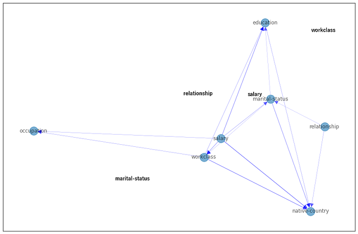
We can now apply the NOTEARS algorithm to learn the structure and visualize the causal model using the plot function. We need to apply thresholding to remove weaker edges and prevent having a fully connected graph. In addition, to avoid spurious edges, constraints on the edges can be included.

# Structure learning
sm = from_pandas(df_num)

# Thresholding
sm.remove_edges_below_threshold(0.8)

# Make plot
plt.figure(figsize=(15,10));
edge_width = [ d['weight']*0.3 for (u,v,d) in sm.edges(data=True)]
nx.draw_networkx(sm, node_size=400, arrowsize=20, alpha=0.6, edge_color='b', width=edge_width)

# If required, remove spurious edges and relearn structure.
sm = from_pandas(df_num, tabu_edges=[("relationship", "native-country")], w_threshold=0.8)

With the derived structure, we can learn the conditional probability distribution (CPDs) and start making queries. However, there are a few additional steps to take, i.e., reducing the cardinality of categorical features and discretizing numeric features. Note that we also need to specify the node states in the form of a dictionary to prevent manually converting numeric values into categorical labels. Although each step is important, for the sake of simplicity, I will skip these steps to avoid many lines of code. For full details, I recommend reading the documentation manual here. It also demonstrates how to use a few helper methods to make discretization easier.

# Step 1: Create a new instance of BayesianNetwork
bn = BayesianNetwork(sm)

# Step 2: Reduce the cardinality of categorical features
# Use domain knowledge or other manners to remove redundant features.

# Step 3: Create Labels for Numeric Features
# Create a dictionary that describes the relation between numeric value and label.

# Step 4: Specify all of the states that each node can take
bn = bn.fit_node_states(df)

# Step 5: Fit Conditional Probability Distributions
bn = bn.fit_cpds(df, method="BayesianEstimator", bayes_prior="K2")

# Return CPD for education
result = bn.cpds["education"]

# Extract any information and probabilities related to education.
print(result)

# marital-status  Divorced              ...   Widowed            
# salary             <=50K              ...      >50K            
# workclass              ? Federal-gov  ... State-gov Without-pay
# education                             ...                      
# 10th            0.077320    0.019231  ...  0.058824      0.0625
# 11th            0.061856    0.012821  ...  0.117647      0.0625
# 12th            0.020619    0.006410  ...  0.058824      0.0625
# 1st-4th         0.015464    0.006410  ...  0.058824      0.0625
# 5th-6th         0.010309    0.006410  ...  0.058824      0.0625
# 7th-8th         0.056701    0.006410  ...  0.058824      0.0625
# 9th             0.067010    0.006410  ...  0.058824      0.0625
# Assoc-acdm      0.025773    0.057692  ...  0.058824      0.0625
# Assoc-voc       0.046392    0.051282  ...  0.058824      0.0625
# Bachelors       0.097938    0.128205  ...  0.058824      0.0625
# Doctorate       0.005155    0.006410  ...  0.058824      0.0625
# HS-grad         0.278351    0.333333  ...  0.058824      0.0625
# Masters         0.015464    0.032051  ...  0.058824      0.0625
# Preschool       0.005155    0.006410  ...  0.058824      0.0625
# Prof-school     0.015464    0.006410  ...  0.058824      0.0625
# Some-college    0.201031    0.314103  ...  0.058824      0.0625
# [16 rows x 126 columns]

Summary

• Input data: The input data set must be discrete. Continuous data is not supported.
• Advantages: Causal networks can be learned, and inferences on the data can be performed.

Disadvantages:

• Requires intensive pre-processing steps. Helper functionalities are provided to reduce the cardinality of categorical features.
• It only supports older versions of Python >=3.6 up to 3.10.
• It only supports older versions of pgmpy ≥ 0.1.14 up to < 0.1.20

For more details, see this blog over here:

4. The DoWhy Library.

DoWhy is a Python library for causal inference that supports explicit modeling and testing of causal assumptions [2, 3]. In comparison to Bnlearn and Pgmpy, in the DoWhy library, it is obligatory to define both the outcome variable and the treatment variable. The treatment variable is the variable of interest that you want to investigate the causal effect of, and the outcome variable is the variable that you want to measure the effect on. In addition, it is also recommended to provide a DAG, aka the causal relationships between the nodes. To create the causal graph for your dataset, you either need domain knowledge or you can connect each variable to the target and treatment variable. Note that the latter is automatically performed when no DAG is given. For this data set, I do not include a known structure and let DoWhy create edges between all variables to the outcome and treatment variable. The first code section shows the required pre-processing steps, and the second code section shows the creation of the causal model.

# Installation
pip install dowhy
# Import libraries
from dowhy import CausalModel
import dowhy.datasets
import datazets as dz
from sklearn.preprocessing import LabelEncoder
import numpy as np
le = LabelEncoder()

# Import data set and drop continous and sensitive features
df = dz.get(data='census_income')

drop_cols = ['age', 'fnlwgt', 'education-num', 'capital-gain', 'capital-loss', 'hours-per-week', 'race', 'sex']
df.drop(labels=drop_cols, axis=1, inplace=True)

# Treatment variable must be binary
df['education'] = df['education']=='Doctorate'

# Next, we need to make our data numeric.
df_num = df.copy()
for col in df_num.columns:
    df_num[col] = le.fit_transform(df_num[col])

# Specify the treatment, outcome, and potential confounding variables
treatment = "education"
outcome = "salary"

# Step 1. Create a Causal Graph
model= CausalModel(
        data=df_num,
        treatment=treatment,
        outcome=outcome,
        common_causes=list(df.columns[~np.isin(df.columns, [treatment, outcome])]),
        graph_builder='ges',
        alpha=0.05,
        )

# Display the model
model.view_model()

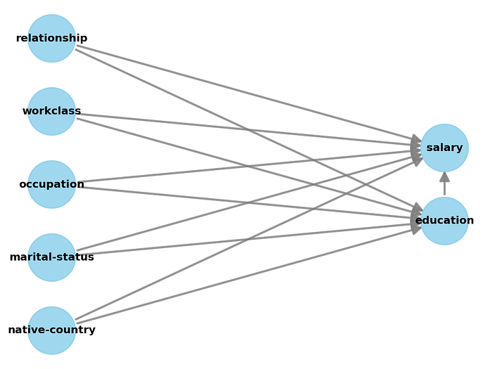
As you may have noticed in the code section above, the treatment variable must be binary (set to Doctorate), and all categorical variables need to be encoded into numeric values. In the code section below we will be using the properties of the causal graph to identify the causal effect. The result may not be surprising. It shows that having a Doctorate increases the chances of a good salary.

# Step 2: Identify causal effect and return target estimands
identified_estimand = model.identify_effect(proceed_when_unidentifiable=True)

# Results
print(identified_estimand)
"""
[16-09-2025 21:06:21] [dowhy.causal_identifier.auto_identifier] [INFO] Causal effect can be identified.
[16-09-2025 21:06:21] [dowhy.causal_identifier.auto_identifier] [INFO] Instrumental variables for treatment and outcome:[]
[16-09-2025 21:06:21] [dowhy.causal_identifier.auto_identifier] [INFO] Frontdoor variables for treatment and outcome:[]
[16-09-2025 21:06:21] [dowhy.causal_identifier.auto_identifier] [INFO] Number of general adjustment sets found: 1
[16-09-2025 21:06:21] [dowhy.causal_identifier.auto_identifier] [INFO] Causal effect can be identified.
"""

print(identified_estimand)

"""
Estimand type: EstimandType.NONPARAMETRIC_ATE

### Estimand : 1
Estimand name: backdoor
Estimand expression:
     d                                                                         ↪
────────────(E[salary|native-country,occupation,marital-status,workclass,relat ↪
d[education]                                                                   ↪

↪          
↪ ionship])
↪          
Estimand assumption 1, Unconfoundedness: If U→{education} and U→salary then P(salary|education,native-country,occupation,marital-status,workclass,relationship,U) = P(salary|education,native-country,occupation,marital-status,workclass,relationship)

### Estimand : 2
Estimand name: iv
No such variable(s) found!

### Estimand : 3
Estimand name: frontdoor
No such variable(s) found!

### Estimand : 4
Estimand name: general_adjustment
Estimand expression:
     d                                                                         ↪
────────────(E[salary|native-country,marital-status,occupation,workclass,relat ↪
d[education]                                                                   ↪

↪          
↪ ionship])
↪          
Estimand assumption 1, Unconfoundedness: If U→{education} and U→salary then P(salary|education,native-country,marital-status,occupation,workclass,relationship,U) = P(salary|education,native-country,marital-status,occupation,workclass,relationship)
"""

# Step 3: Estimate the target estimand using a statistical method.
estimate = model.estimate_effect(identified_estimand, method_name="backdoor.propensity_score_stratification"

# Results
print(estimate)
"""
*** Causal Estimate ***

## Identified estimand
Estimand type: EstimandType.NONPARAMETRIC_ATE

### Estimand : 1
Estimand name: backdoor
Estimand expression:
     d                                                                         ↪
────────────(E[salary|native-country,occupation,marital-status,workclass,relat ↪
d[education]                                                                   ↪

↪          
↪ ionship])
↪          
Estimand assumption 1, Unconfoundedness: If U→{education} and U→salary then P(salary|education,native-country,occupation,marital-status,workclass,relationship,U) = P(salary|education,native-country,occupation,marital-status,workclass,relationship)

## Realized estimand
b: salary~education+native-country+occupation+marital-status+workclass+relationship
Target units: ate

## Estimate
Mean value: 0.46973242081553496
## Estimate
# Mean value: 0.4697157228651772

"""
# Step 4: Refute the obtained estimate using multiple robustness checks.
refute_results = model.refute_estimate(identified_estimand, estimate, method_name="random_common_cause")

Summary

• Input data: Outcome variable and Treatment variable. It is highly recommended to provide a causal DAG.
• Requirements: The treatment variable must be binary, and all categorical variables need to be encoded into numeric values.
• Disadvantage: The output contains text and other details, which complicates how to interpret the results. It can also not learn the causal DAG from the data.

For more details, see the blog for DoWhy:

5. The PyAgrum Library.

PyAgrum is a Python library for probabilistic graphical models that provides tools for learning, analyzing, and visualizing Bayesian networks. It supports a broad range of models that also includes Markov random models on top of the Bayesian models. In line with the other libraries, it also offers multiple structure learning algorithms (e.g., Hill-Climbing, Chow-Liu, K2) and scoring functions (e.g., BIC, AIC) to infer causal relationships from data. Users can also incorporate expert knowledge in the form of DAGs or constraints to guide the learning process.

In PyAgrum, the learner requires a fully discrete dataset and does not handle missing values natively, so preprocessing steps such as converting variables to categorical types or replacing unknowns are necessary. Once the dataset is prepared, you can define a learner, select a scoring method and search algorithm, and run structure learning to obtain a Bayesian network. The network can then be inspected, queried, or used for further inference and decision analysis. For practical use, PyAgrum provides rich visualization and analysis tools. In the following code section, we handle the cleaning of the data set, preprocessing, and categorical conversion. After these steps, we can learning the network and visualize the structure.

# Install pyagrum
pip install pyagrum

# Install graphviz (needed for visualizations)
pip install setgraphviz
import datazets as dz
import pandas as pd
import pyagrum as gum
import pyagrum.lib.notebook as gnb
import pyagrum.lib.explain as explain
import pyagrum.lib.bn_vs_bn as bnvsbn

# Import library to show the dot graphs
from setgraphviz import setgraphviz
# Set path
setgraphviz()

# Import data set and drop continous and sensitive features
df = dz.get(data='census_income')
# Data cleaning
drop_cols = ['age', 'fnlwgt', 'education-num', 'capital-gain', 'capital-loss', 'hours-per-week', 'race', 'sex']
df.drop(labels=drop_cols, axis=1, inplace=True)
# Drop rows with any missing values
df2 = df.dropna().copy()
# Replace *all* missing values with a placeholder string
df2 = df2.fillna("missing").replace("?", "missing")

# Make sure categorical columns are categorical dtype (pyAgrum expects discrete variables)
for col in df2.columns:
    df2[col] = df2[col].astype("category")
          
# Create the learner from the pandas DataFrame
learner = gum.BNLearner(df2)

# Configure score and search
learner.useScoreBIC()
learner.useGreedyHillClimbing()

# Learn the network
bn = learner.learnBN()

# Learn the parameters
bn2 = learner.learnParameters(bn.dag())

# Plot the network
gnb.showBN(bn2)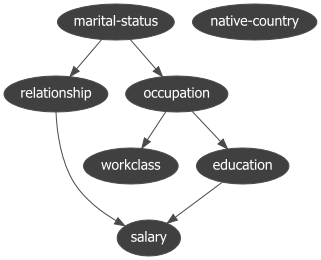

Summary

• Input data: A fully discrete dataset (all variables categorical or integer-coded). Optional: a DAG or constraints to guide structure learning.
• Requirements: No missing values allowed. All categorical variables must be encoded as category or integer codes.
• Disadvantage: Cannot handle missing data natively. For continuous variables, discretization is required. Visualization and interpretation may require additional steps or external tools like Graphviz.

6. The CausalImpact Library.

CausalImpact is a Python package for causal inference using Bayesian structural time-series models [4]. The main goal is to infer the expected effect of a given intervention by analyzing differences between expected and observed time series data, such as Program Evaluation or Treatment Effect Analysis. It makes the assumption that the response variable can be precisely modeled by linear regression. However, it must not be affected by the intervention that took place. For instance, if a company wants to infer what impact a given marketing campaign will have on its "revenue", then its daily "visits" cannot be used as a covariate, as the total visits might be affected by the campaign. In the following example, we will create 100 observations with a response variable y and a predictor x1. Note that in real use cases, we will have many more predictor variables. For demonstration, the intervention effect is created by changing the response variable by 10 units after time point 71.

To estimate the causal effect, we first need to specify the pre-intervention period and the post-intervention period. With the run function, we fit a time series model using MLE (default), and estimate the causal effect.

# Installation
pip install causalimpact
# Import libraries
import numpy as np
import pandas as pd
from statsmodels.tsa.arima_process import arma_generate_sample
import matplotlib.pyplot as plt
from causalimpact import CausalImpact

# Generate samples
x1 = arma_generate_sample(ar=[0.999], ma=[0.9], nsample=100) + 100
y = 1.2 * x1 + np.random.randn(100)
y[71:] = y[71:] + 10
data = pd.DataFrame(np.array([y, x1]).T, columns=["y","x1"])

# Initialize
impact = CausalImpact(data, pre_period=[0,69], post_period=[71,99])

# Create inferences
impact.run()

# Plot
impact.plot()

# Results
impact.summary()
#                              Average    Cumulative
# Actual                           130          3773
# Predicted                        120          3501
# 95% CI                    [118, 122]  [3447, 3555]
                                                  
# Absolute Effect                    9           272
# 95% CI                       [11, 7]    [326, 218]
                                                  
# Relative Effect                 7.8%          7.8%
# 95% CI                  [9.3%, 6.2%]  [9.3%, 6.2%]
                                                  
# P-value                         0.0%              
# Prob. of Causal Effect        100.0%

# Summary report
impact.summary(output="report")

The Average column describes the average time during the post-intervention period. The Cumulative column sums up individual time points, which is a useful perspective if the response variable represents a flow quantity, such as queries, clicks, visits, installs, sales, or revenue. We see that in this example, there is a 100% probability of causal effect with a P-value of 0 which is correct because we included this in the data.

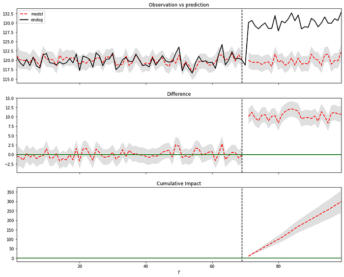
In the plot (Figure 4), we can see three panels that can be described as follows: In Panel 1, we can see the data along with a counterfactual prediction specifically for the post-treatment period. In the second panel, the difference between the observed data and the counterfactual predictions is shown. This difference represents the estimated pointwise causal effect, as determined by the model. The bottom panel depicts the cumulative effect of the intervention by aggregating the pointwise contributions from the previous panel. It is important to note that the validity of these inferences relies on the assumption that the covariates were not influenced by the intervention itself. Additionally, the model assumes that the relationship established between the covariates and the treated time series during the pre-period remains consistent throughout the post-period.

Summary

• Input data: Time series data.
• Requirements: The pre-intervention period and post-intervention period need to be specified.
• Advantage: Can determine the causal effects on time-series data.
• Disadvantage: Requires pandas<2.0

For more details, see this blog over here:

Summary Between The Libraries.

We have compared six libraries for learning causality, each with its own (dis)advantages and its focus on solving certain problems. The BnLearn library is suited in use cases where you have discrete, mixed, or continuous data sets and need to derive the causal DAG from the data (structure learning), do parameter learning (CPD estimations), or in cases where you aim to make inferences (do-calculus). The advantages are that many pre- and post-processing steps are solved within the pipelines which makes it less error-prone. It allows categorical (string) labels as input and can remove spurious edges using statistical tests (independence test). In addition, edges or nodes can also be whitelisted or blacklisted. Another important aspect is that it is compatible with the latest libraries, among others, numpy and pandas.

The Pgmpy library contains low-level statistical functions to create and combine various methods for structure learning, parameter learning, and inference. It is flexible in usage but requires good knowledge of Bayesian modeling. Note that the Bnlearn library utilizes some functions from Pgmpy and has therefore overlapping functionality. Or in other words, if you aim to create customized pipelines, it is recommended to use Pgmpy. Otherwise, I recommend using bnlearn.

The CausalNex library can be used to derive the causal DAG from the data, and make inferences. Note that it only works on discrete data sets. After detecting a causal DAG, edges can be removed by thresholding. Unfortunately, it can not work with categorical labels and needs to be converted into numerical values. In addition, various intermediate preprocessing steps are required. For example, reducing the cardinality of categorical features, describing numeric features, and specifying all of the states that each node can take in the form of a dictionary. Although this gives more control to the user in the modeling part, the extra modeling adds a layer of complexity. Finally, it is not compatible with Python version > 3.10 and also not compatible with the latest numpy version.

The DoWhy approach is a good choice in cases where you want to estimate the causal effect if you have an outcome variable together with a treatment variable. Ideal for use cases where you need A/B testing, such as determining the causes of hotel booking cancellations. The outcome can be set as "cancelation", and treatment can be set as "different room assigned". Another use case could be to estimate the effect of a member rewards program. Note that this library is not designed to learn the causal DAG from the data. However, it does need a causal DAG as input for the model which you need to provide manually.

CausalImpact is a Python package for causal inference using Bayesian structural time-series models. Although it also computes causality, it is not comparable in functionality to the other libraries as it does not intend to create a causal DAG or make inferences on the data. The goal is to infer the expected effect of a given intervention by analyzing differences between expected and observed time series data, such as Program Evaluation or Treatment Effect Analysis.

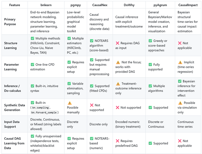
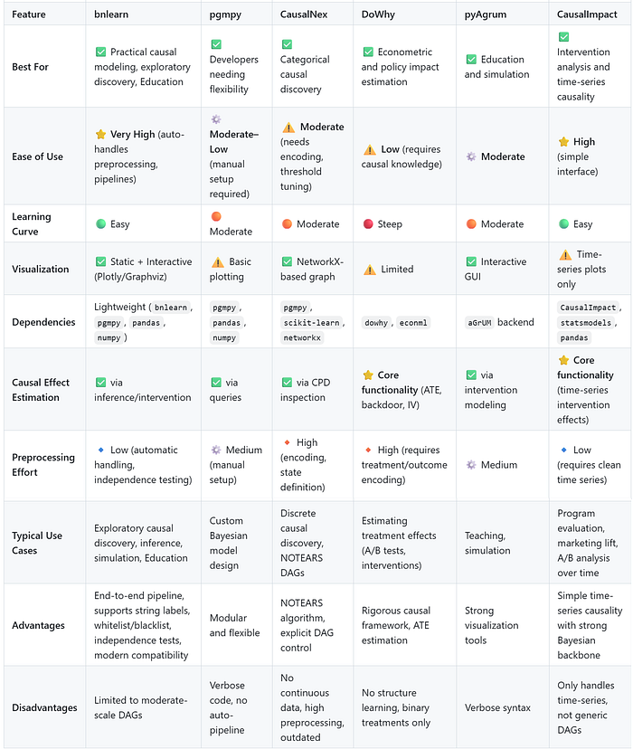
Table Comparison.

I summarized all results in two tables, the first one compares the functions, and the second table compares the generic usage:

Final words.

Modeling your data for causality can be challenging for many reasons. It starts with choosing the right library that matches your specific use case, for which we have seen a comparison of six popular causal inference libraries: Bnlearn, Pgmpy, CausalNex, DoWhy, Pyagrum, and CausalImpact. Each library has its own (dis)advantages and is best suited for certain use cases. The libraries are compared in their functionalities, capabilities, and interpretability of the results using the same data set. Only for CausalImpact, a different data set is used, as it could only model continuous values and required time series data.

A grouping on functionality would cluster Bnlearn, Pgmpy, Pyagrum and CausalNex as they contain functionalities for structure learning, parameter learning, and making inferences. The second group is DoWhy and CausalImpact, which are designed to measure the causal effect of treatment variable(s) on an outcome variable Y, controlling for a set of features X. Besides the six causal libraries described here, more libraries are worth looking at, such as EconML, Pyro, and CausalML, which fall in the second group (causal effect of treatment variable on an outcome variable).

Be Safe. Stay Frosty.

Cheers E.

I hope you enjoyed reading this blog. You are welcome to follow me because I write more about data science! Also, try the hands-on examples in this blog. This will help you to learn quicker, understand better, and remember longer. Grab a coffee and have fun! Disclaimer: I am the developer of the Python bnlearn library. I tried to make the comparison as honest as possible. Whatever your decision for a causal library is, make sure you fully understand the modeling part and can interpret the results.

Software

• Bnlearn Colab Notebook examples

Let's connect!

• Let's connect on LinkedIn
• Follow me on Github
• Follow me on Medium

References

1. Census Income. (1996). UCI Machine Learning Repository. https://doi.org/10.24432/C5S595.
2. E. Taskesen, Synthetic Data: The Essentials Of Data Generation Using Bayesian Sampling., Data Science Collective (DSC), May 2025
3. E. Taskesen, Why Prediction Isn't Enough: Using Bayesian Models to Change the Outcome., Towards Data Science (TDS), June 2025
4. Dowhy: https://www.pywhy.org/dowhy/v0.8/getting_started/intro.html
5. Amit Sharma, Emre Kiciman. DoWhy: An End-to-End Library for Causal Inference. 2020. https://arxiv.org/abs/2011.04216
6. Kay H. et al, Inferring causal impact using Bayesian structural time-series models, 2015, Annals of Applied Statistics (247–274, vol9)
7. Xun Zheng et al, DAGs with NO TEARS: Continuous Optimization for Structure Learning, 32nd Conference on Neural Information Processing Systems (NeurIPS 2018), Montréal, Canada.
8. AI4I 2020 Predictive Maintenance Dataset. (2020). UCI Machine Learning Repository.
9. PyAgrum: Python Library for Probabilistic Graphical Models. Available at: https://pyagrum.readthedocs.io.
10. E. Taskesen, The Starters Guide to Causal Structure Learning with Bayesian Methods in Python, Data Science Collective (DSC), September 2025
11. A. Ankan, Causal Discovery with Mixed Data using pgmpy, Medium, February 2025
12. QuantumBlack, AI by McKinsey, Introducing CausalNex — Driving Models Which Respect Cause And Effect, Medium, January 2020
13. Chris, Causal Inference with Python –Introduction to DoWhy, Medium, May 2025
14. Juan Jose Munoz, Unlock Your Full Potential as a Business Analyst With the Powerful 5-Step Causal Impact Framework, Medium, November 2023