The Starters Guide to Causal Structure Learning with Bayesian Methods in Python.

Hands-on Tutorials

Determining causality across variables can be a challenging step, not only in modeling but also in understanding the required steps and their interpretation. In this blog, you will first learn some key background concepts of causal models within the framework of Bayesian probability. With this foundation, we then move to the second part, where you will learn how to detect causal relationships using Bayesian structure learning. To illustrate the concepts, we use a small, well-known dataset (the sprinkler dataset), which helps to clearly demonstrate how structures are learned. All analyses are carried out using the Python library bnlearn.

If you found this article helpful, you are welcome to follow me because I write more about Bayesian statistics! I recommend experimenting with the hands-on examples in this blog. This will help you to learn quicker, understand better, and remember longer. Grab a coffee and have fun!

The Background That You Need To Know.

The use of machine learning techniques has become a standard toolkit to obtain useful insights and make predictions in many areas, such as disease prediction, recommendation systems, and natural language processing. Although good performances can be achieved, it is not straightforward to extract causal relationships with, for example, the target variable. In other words, which variables do have direct causal effect on the target variable? Such insights are important to determine the driving factors that reach the conclusion, and as such, strategic actions can be taken. A branch of machine learning is Bayesian probabilistic graphical models, also named Bayesian networks (BN), which can be used to determine such causal factors. Note that a lot of aliases exist for Bayesian graphical models, such as: Bayesian networks, Bayesian belief networks, Bayes Net, causal probabilistic networks, and Influence diagrams.

Let's rehash some terminology before we jump into the technical details of causal models. It is common to use the terms "correlation" and "association" interchangeably. But we all know that correlation or association is not causation. Or in other words, observed relationships between two variables do not necessarily mean that one causes the other. Technically, correlation refers to a linear relationship between two variables, whereas association refers to any relationship between two (or more) variables. Causation, on the other hand, means that one variable (often called the predictor variable or independent variable) causes the other (often called the outcome variable or dependent variable) [1]. In the next two sections, I will briefly describe correlation and association by example in the next section.

Warming Up: Correlation Is Not …

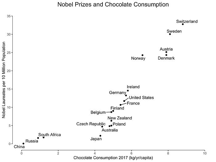
Pearson's correlation is the most commonly used correlation coefficient. It is so common that it is often used synonymously with correlation. The strength is denoted by r and measures the strength of a linear relationship in a sample on a standardized scale from -1 to 1. There are three possible results when using correlation:

• Positive correlation: a relationship between two variables in which both variables move in the same direction
• Negative correlation: a relationship between two variables in which an increase in one variable is associated with a decrease in the other, and
• No correlation: when there is no relationship between two variables.

An example of positive correlation is demonstrated in Figure 1, where the relationship is seen between chocolate consumption and the number of Nobel Laureates per country [2].

But What Is Association?

When we talk about association, we mean that certain values of one variable tend to co-occur with certain values of the other variable. From a statistical point of view, there are many measures of association, such as the chi-square test, Fisher's exact test, hypergeometric test, etc. Association measures are used when one or both variables are categorical, that is, either nominal or ordinal. It should be noted that correlation is a technical term, whereas the term association is not, and therefore, there is not always consensus about the meaning in statistics. This means that it's always a good practice to state the meaning of the terms you're using. More information about associations can be found in this blog [4], and read this blog for more details about exploring and understanding your data with a network of significant associations [5].

Example: Determine the Associations

To demonstrate the use of associations, I will use the Hypergeometric test and quantify whether two variables are associated in the predictive maintenance data set [9] (CC BY 4.0 licence). The predictive maintenance data set is a so-called mixed-type data set containing a combination of continuous, categorical, and binary variables. It captures operational data from machines, including both sensor readings and failure events. The data set also records whether specific types of failures occurred, such as tool wear failure or heat dissipation failure, represented as binary variables. See the table below with details about the variables.

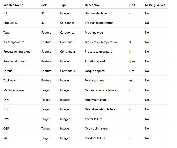
One of the most important variables is machine failure and power failure. We would expect a strong association between these two variables. Let me demonstrate how to compute the association between the two. First, we need to install the bnlearn library and load the data set.

# Install Python bnlearn package
pip install bnlearn
import bnlearn
import pandas as pd
from scipy.stats import hypergeom

# Load predictive maintenance data set
df = bnlearn.import_example(data='predictive_maintenance')

# print dataframe
print(df)
+-------+------------+------+------------------+----+-----+-----+-----+-----+
|  UDI | Product ID  | Type | Air temperature  | .. | HDF | PWF | OSF | RNF |
+-------+------------+------+------------------+----+-----+-----+-----+-----+
|    1 | M14860      |   M  | 298.1            | .. |   0 |   0 |   0 |   0 |
|    2 | L47181      |   L  | 298.2            | .. |   0 |   0 |   0 |   0 |
|    3 | L47182      |   L  | 298.1            | .. |   0 |   0 |   0 |   0 |
|    4 | L47183      |   L  | 298.2            | .. |   0 |   0 |   0 |   0 |
|    5 | L47184      |   L  | 298.2            | .. |   0 |   0 |   0 |   0 |
| ...  | ...         | ...  | ...              | .. | ... | ... | ... | ... |
| 9996 | M24855      |   M  | 298.8            | .. |   0 |   0 |   0 |   0 |
| 9997 | H39410      |   H  | 298.9            | .. |   0 |   0 |   0 |   0 |
| 9998 | M24857      |   M  | 299.0            | .. |   0 |   0 |   0 |   0 |
| 9999 | H39412      |   H  | 299.0            | .. |   0 |   0 |   0 |   0 |
|10000 | M24859      |   M  | 299.0            | .. |   0 |   0 |   0 |   0 |
+-------+-------------+------+------------------+----+-----+-----+-----+-----+
[10000 rows x 14 columns]

Null hypothesis: There is no association between machine failure and power failure (PWF).

print(df[['Machine failure','PWF']])

| Index | Machine failure | PWF |
|-------|------------------|-----|
| 0     | 0                | 0   |
| 1     | 0                | 0   |
| 2     | 0                | 0   |
| 3     | 0                | 0   |
| 4     | 0                | 0   |
| ...   | ...              | ... |
| 9995  | 0                | 0   |
| 9996  | 0                | 0   |
| 9997  | 0                | 0   |
| 9998  | 0                | 0   |
| 9999  | 0                | 0   |
|-------|------------------|-----|

# Total number of samples
N=df.shape[0]

# Number of success in the population
K=sum(df['Machine failure']==1)

# Sample size/number of draws
n=sum(df['PWF']==1)

# Overlap between Power failure and machine failure
x=sum((df['PWF']==1) & (df['Machine failure']==1))

print(x-1, N, n, K)
# 94 10000 95 339

# Compute
P = hypergeom.sf(x, N, n, K)
P = hypergeom.sf(94, 10000, 95, 339)

print(P)
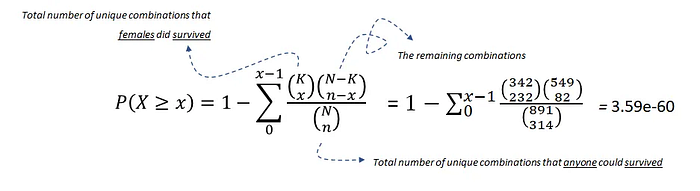
# 1.669e-146

The hypergeometric test uses the hypergeometric distribution to measure the statistical significance of a discrete probability distribution. In this example, N is the population size (10000), K is the number of successful states in the population (339), n is the sample size/number of draws (95), and x is the number of successes (94).

We can reject the null hypothesis under alpha=0.05, and therefore, we can speak about a statistically significant association between machine failure and power failure. Importantly, association by itself does not imply causation. Strictly speaking, this statistic also does not tell us the direction of impact. We need to distinguish between marginal associations and conditional associations. The latter is the key building block of causal inference. Now that we have learned about associations, we can continue to causation in the next section!

This Is Causation.

Causation means that one (independent) variable causes the other (dependent) variable and is formulated by Reichenbach (1956) as follows:

If two random variables X and Y are statistically dependent (X/Y), then either (a) X causes Y, (b) Y causes X, or (c ) there exists a third variable Z that causes both X and Y. Further, X and Y become independent given Z, i.e., X⊥Y∣Z.

This definition is incorporated in Bayesian graphical models. To explain this more thoroughly, let's start with the graph and visualize the statistical dependencies between the three variables described by Reichenbach (X, Y, Z) as shown in Figure 2. Nodes correspond to variables (X, Y, Z), and the directed edges (arrows) indicate dependency relationships or conditional distributions.

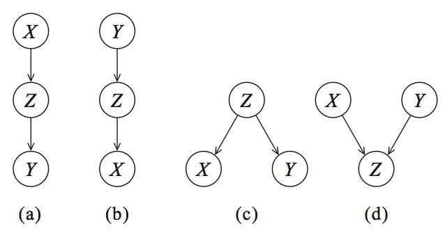
Four graphs can be created: (a) and (b) are cascade, © common parent, and (d) the V-structure. These four graphs form the basis for every Bayesian network.

1. How can we tell what causes what?

The conceptual idea to determine the direction of causality, thus which node influences which node, is by holding one node constant and then observing the effect. As an example, let's take DAG (a) in Figure 2, which describes that Z is caused by X, and Y is caused by Z. If we now keep Z constant, there should not be a change in Y if this model is true. Every Bayesian network can be described by these four graphs, and with probability theory (see the section below) we can glue the parts together.

Bayesian network is a happy marriage between probability and graph theory.

It should be noted that a Bayesian network is a Directed Acyclic Graph (DAG), and DAGs are causal. This means that the edges in the graph are directed and there is no (feedback) loop (acyclic).

2. Probability theory.

Probability theory, or more specifically, Bayes' theorem or Bayes Rule, forms the fundament for Bayesian networks. The Bayes' rule is used to update model information, and stated mathematically as the following equation:

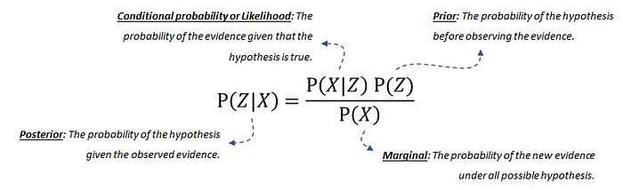
The equation consists of four parts;

• The posterior probability is the probability that Z occurs given X.
• The conditional probability or likelihood is the probability of the evidence given that the hypothesis is true. This can be derived from the data.
• Our prior belief is the probability of the hypothesis before observing the evidence. This can also be derived from the data or domain knowledge.
• The marginal probability describes the probability of the new evidence under all possible hypotheses, which needs to be computed.

If you want to read more about the (factorized) probability distribution or more details about the joint distribution for a Bayesian network, try this blog [6].

3. Bayesian Structure Learning to estimate the DAG.

With structure learning, we want to determine the structure of the graph that best captures the causal dependencies between the variables in the data set. Or in other words:

Structure learning is to determine the DAG that best fits the data.

A naïve manner to find the best DAG is by simply creating all possible combinations of the graph, i.e., by making tens, hundreds, or even thousands of different DAGs until all combinations are exhausted. Each DAG can then be scored on the fit of the data. Finally, the best-scoring DAG is returned. In the case of variables X, Y, Z, one can make the graphs as shown in Figure 2 and a few more, because it is not only X>Z>Y (Figure 2a), but it can also be Z>X>Y, etc. The variables X, Y, Z can be boolean values (True or False), but can also have multiple states. In the latter case, the search space of DAGs becomes so-called super-exponential in the number of variables that maximize the score. This means that an exhaustive search is practically infeasible with a large number of nodes, and therefore, various greedy strategies have been proposed to browse DAG space. With optimization-based search approaches, it is possible to browse a larger DAG space. Such approaches require a scoring function and a search strategy. A common scoring function is the posterior probability of the structure given the training data, like the BIC or the BDeu.

Structure learning for DAGs requires two components: 1. scoring function and 2. search strategy.

Before we jump into the examples, it is always good to understand when to use which technique. There are two broad approaches to search throughout the DAG space and find the best-fitting graph for the data.

• Score-based structure learning
• Constraint-based structure learning

Note that a local search strategy makes incremental changes aimed at improving the score of the structure. A global search algorithm like Markov chain Monte Carlo can avoid getting trapped in local minima, but I will not discuss that here.

4. Score-based Structure Learning.

Score-based approaches have two main components:

1. The search algorithm to optimize throughout the search space of all possible DAGs, such as ExhaustiveSearch, Hillclimbsearch, Chow-Liu.
2. The scoring function indicates how well the Bayesian network fits the data. Commonly used scoring functions are Bayesian Dirichlet scores such as BDeu or K2 and the Bayesian Information Criterion (BIC, also called MDL).

Four common score-based methods are depicted below, but more details about the Bayesian scoring methods can be found here [11].

• ExhaustiveSearch, as the name implies, scores every possible DAG and returns the best-scoring DAG. This search approach is only attractive for very small networks and prohibits efficient local optimization algorithms to always find the optimal structure. Thus, identifying the ideal structure is often not tractable. Nevertheless, heuristic search strategies often yield good results if only a few nodes are involved (read: less than 5 or so).
• Hillclimbsearch is a heuristic search approach that can be used if more nodes are used. HillClimbSearch implements a greedy local search that starts from the DAG "start" (default: disconnected DAG) and proceeds by iteratively performing single-edge manipulations that maximally increase the score. The search terminates once a local maximum is found.
• Chow-Liu algorithm is a specific type of tree-based approach. The Chow-Liu algorithm finds the maximum-likelihood tree structure where each node has at most one parent. The complexity can be limited by restricting to tree structures.
• Tree-augmented Naive Bayes (TAN) algorithm is also a tree-based approach that can be used to model huge data sets involving lots of uncertainties among its various interdependent feature sets [6].

5. Constraint-based Structure Learning

Chi-square test. A different, but quite straightforward approach to construct a DAG by identifying independencies in the data set using hypothesis tests, such as the chi2 test statistic. This approach does rely on statistical tests and conditional hypotheses to learn independence among the variables in the model. The P-value of the chi2 test is the probability of observing the computed chi2 statistic, given the null hypothesis that X and Y are independent, given Z. This can be used to make independent judgments, at a given level of significance. An example of a constraint-based approach is the PC algorithm, which starts with a complete, fully connected graph and removes edges based on the results of the tests if the nodes are independent until a stopping criterion is achieved.

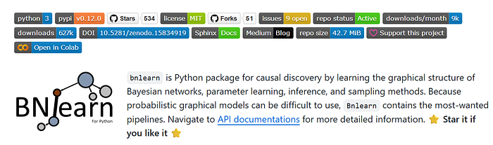
The bnlearn library

A few words about the bnlearn library that is used for all the analysis in this article. The bnlearn library provides tools for creating, analyzing, and visualizing Bayesian networks in Python. It supports discrete, mixed, and continuous datasets and is designed to be easy to use while including the most essential Bayesian pipelines for causal learning. With bnlearn, you can perform structure learning, parameter estimation, inference, and create synthetic data, making it suitable for both exploratory analysis and advanced causal discovery. A range of statistical tests can be applied simply by specifying parameters during initialization. Additional helper functions allow you to transform datasets, derive the topological ordering of an entire graph, compare two networks, and generate a wide variety of insightful plots. Core functionalities include:

The key pipelines are:

• Structure Learning: Learn the network structure from data or integrate expert knowledge.
• Parameter Learning: Estimate conditional probability distributions from observed data.
• Inference: Query the network to compute probabilities, simulate interventions, and test causal effects.
• Synthetic Data: Generate new datasets from learned Bayesian networks for simulation, benchmarking, or data augmentation.
• Discretize Data: Transform continuous variables into discrete states using built-in discretization methods for easier modeling and inference.
• Model Evaluation: Compare networks using scoring functions, statistical tests, and performance metrics.
• Visualization: Interactive graph plotting, probability heatmaps, and structure overlays for transparent analysis.

In this article, I don't mention synthetic data, but if you want to learn more about data generation, I recommend reading these blogs for more details:

What benefits does bnlearn offer over other Bayesian analysis implementations?

• Contains the most-wanted Bayesian pipelines.
• Simple and intuitive in usage.
• Open-source with MIT Licence.
• Documentation page and blogs.
• +500 stars on Github with over 600K downloads.

Structure Learning.

To learn the fundamentals of causal structure learning, we will start with a small and intuitive example. Suppose you have a sprinkler system in your backyard and for the last 1000 days, you measured four variables, each with two states: Rain (yes or no), Cloudy (yes or no), Sprinkler system (on or off), and Wet grass (true or false). Based on these four variables and your conception of the real world, you may have an intuition of how the graph should look like, right? If not, it is good that you read this article because with structure learning you will find out!

With bnlearn for Python it is easy to determine the causal relationships with only a few lines of code.

In the example below, we will import the bnlearn library for Python, and load the sprinkler data set. Then we can determine which DAG fits the data best. Note that the sprinkler data set is readily cleaned without missing values, and all values have the state 1 or 0.

# Import bnlearn package
import bnlearn as bn

# Load sprinkler data set
df = bn.import_example('sprinkler')

# Print to screen for illustration
print(df)
'''
+----+----------+-------------+--------+-------------+
|    |   Cloudy |   Sprinkler |   Rain |   Wet_Grass |
+====+==========+=============+========+=============+
|  0 |        0 |           0 |      0 |           0 |
+----+----------+-------------+--------+-------------+
|  1 |        1 |           0 |      1 |           1 |
+----+----------+-------------+--------+-------------+
|  2 |        0 |           1 |      0 |           1 |
+----+----------+-------------+--------+-------------+
| .. |        1 |           1 |      1 |           1 |
+----+----------+-------------+--------+-------------+
|999 |        1 |           1 |      1 |           1 |
+----+----------+-------------+--------+-------------+
'''

# Learn the DAG in data using Bayesian structure learning:
DAG = bn.structure_learning.fit(df)

# print adjacency matrix
print(DAG['adjmat'])
# target     Cloudy  Sprinkler   Rain  Wet_Grass
# source                                        
# Cloudy      False      False   True      False
# Sprinkler    True      False  False       True
# Rain        False      False  False       True
# Wet_Grass   False      False  False      False

# Plot in Python
G = bn.plot(DAG)

# Make interactive plot in HTML
G = bn.plot(DAG, interactive=True)

# Make PDF plot
bn.plot_graphviz(model)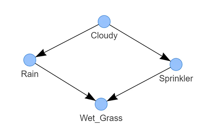

That's it! We have the learned structure as shown in Figure 3. The detected DAG consists of four nodes that are connected through edges, each edge indicates a causal relation. The state of Wet grass depends on two nodes, Rain and Sprinkler. The state of Rain is conditioned by Cloudy, and separately, the state Sprinkler is also conditioned by Cloudy. This DAG represents the (factorized) probability distribution, where S is the random variable for sprinkler, R for the rain, G for the wet grass, and C for cloudy.

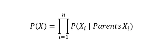
By examining the graph, you quickly see that the only independent variable in the model is C. The other variables are conditioned on the probability of cloudy, rain, and/or the sprinkler. In general, the joint distribution for a Bayesian Network is the product of the conditional probabilities for every node given its parents:

The default setting in bnlearn for structure learning is the hillclimbsearch method and BIC scoring. Notably, different methods and scoring types can be specified. See the examples in the code block below of the various structure learning methods and scoring types in bnlearn:

import bnlearn as bn
# Load sprinkler dataset
df = bn.import_example('sprinkler')

# 'hc' or 'hillclimbsearch'
model_hc_bic  = bn.structure_learning.fit(df, methodtype='hc', scoretype='bic')
model_hc_k2   = bn.structure_learning.fit(df, methodtype='hc', scoretype='k2')
model_hc_bdeu = bn.structure_learning.fit(df, methodtype='hc', scoretype='bdeu')

# 'ex' or 'exhaustivesearch'
model_ex_bic  = bn.structure_learning.fit(df, methodtype='ex', scoretype='bic')
model_ex_k2   = bn.structure_learning.fit(df, methodtype='ex', scoretype='k2')
model_ex_bdeu = bn.structure_learning.fit(df, methodtype='ex', scoretype='bdeu')

# 'cs' or 'constraintsearch'
model_cs_k2   = bn.structure_learning.fit(df, methodtype='cs', scoretype='k2')
model_cs_bdeu = bn.structure_learning.fit(df, methodtype='cs', scoretype='bdeu')
model_cs_bic  = bn.structure_learning.fit(df, methodtype='cs', scoretype='bic')

# 'cl' or 'chow-liu' (requires setting root_node parameter)
model_cl      = bn.structure_learning.fit(df, methodtype='cl', root_node='Wet_Grass')

Although the detected DAG for the sprinkler data set is insightful and shows the causal dependencies for the variables in the data set, it does not allow you to ask all kinds of questions, such as:

How probable is it to have wet grass given the sprinkler is off?

How probable is it to have a rainy day given the sprinkler is off and it is cloudy?

In the sprinkler data set, it may be evident what the outcome is because of your knowledge about the world and logical thinking. But once you have larger, more complex graphs, it may not be so evident anymore. With so-called inferences, we can answer "what-if-we-did-x" type questions that would normally require controlled experiments and explicit interventions to answer.

To make inferences, we need two ingredients: the DAG and Conditional Probabilistic Tables (CPTs). At this point, we have the data stored in the data frame (df), and we have readily computed the DAG. The CPTs can be computed using Parameter learning, and will describe the statistical relationship between each node and its parents. Keep on reading in the next section about parameter learning, and after that, we can start making inferences.

Parameter learning.

Parameter learning is the task of estimating the values of the Conditional Probability Tables (CPTs). The bnlearn library supports Parameter learning for discrete and continuous nodes:

• Maximum Likelihood Estimation is a natural estimate by using the relative frequencies with which the variable states have occurred. When estimating parameters for Bayesian networks, lack of data is a frequent problem and the ML estimator has the problem of overfitting to the data. In other words, if the observed data is not representative (or too small) for the underlying distribution, ML estimations can be extremely far off. As an example, if a variable has 3 parents that can each take 10 states, then state counts will be done separately for 1⁰³ = 1000 parent configurations. This can make MLE very fragile for learning Bayesian Network parameters. A way to mitigate MLE's overfitting is Bayesian Parameter Estimation.
• Bayesian Estimation starts with readily existing prior CPTs, which express our beliefs about the variables before the data was observed. Those "priors" are then updated using the state counts from the observed data. One can think of the priors as consisting of pseudo-state counts, which are added to the actual counts before normalization. A very simple prior is the so-called K2 prior, which simply adds "1" to the count of every single state. A somewhat more sensible choice of prior is BDeu (Bayesian Dirichlet equivalent uniform prior).

Parameter Learning on the Sprinkler Data set.

We will use the Sprinkler data set to learn its parameters. The output of Parameter Learning is the Conditional Probabilistic Tables (CPTs). To learn parameters, we need a Directed Acyclic Graph (DAG) and a data set with the same variables. The idea is to connect the data set with the DAG. In the previous example, we readily computed the DAG (Figure 3). You can use it in this example or alternatively, you can create your own DAG based on your knowledge of the world! In the example, I will demonstrate how to create your own DAG, which can be based on expert/domain knowledge.

import bnlearn as bn

# Load sprinkler data set
df = bn.import_example('sprinkler')

# The edges can be created using the available variables.
print(df.columns)
# ['Cloudy', 'Sprinkler', 'Rain', 'Wet_Grass']

# Define the causal dependencies based on your expert/domain knowledge.
# Left is the source, and right is the target node.
edges = [('Cloudy', 'Sprinkler'),
         ('Cloudy', 'Rain'),
         ('Sprinkler', 'Wet_Grass'),
         ('Rain', 'Wet_Grass')]

# Create the DAG. If not CPTs are present, bnlearn will auto generate placeholders for the CPTs.
DAG = bn.make_DAG(edges)

# Plot the DAG. This is identical as shown in Figure 3
bn.plot(DAG)

# Parameter learning on the user-defined DAG and input data using maximumlikelihood
model = bn.parameter_learning.fit(DAG, df, methodtype='ml')

# Print the learned CPDs
bn.print_CPD(model)

"""
[bnlearn] >[Conditional Probability Table (CPT)] >[Node Sprinkler]:
+--------------+--------------------+------------+
| Cloudy       | Cloudy(0)          | Cloudy(1)  |
+--------------+--------------------+------------+
| Sprinkler(0) | 0.4610655737704918 | 0.91015625 |
+--------------+--------------------+------------+
| Sprinkler(1) | 0.5389344262295082 | 0.08984375 |
+--------------+--------------------+------------+

[bnlearn] >[Conditional Probability Table (CPT)] >[Node Rain]:
+---------+---------------------+-------------+
| Cloudy  | Cloudy(0)           | Cloudy(1)   |
+---------+---------------------+-------------+
| Rain(0) | 0.8073770491803278  | 0.177734375 |
+---------+---------------------+-------------+
| Rain(1) | 0.19262295081967212 | 0.822265625 |
+---------+---------------------+-------------+

[bnlearn] >[Conditional Probability Table (CPT)] >[Node Wet_Grass]:
+--------------+--------------+-----+----------------------+
| Rain         | Rain(0)      | ... | Rain(1)              |
+--------------+--------------+-----+----------------------+
| Sprinkler    | Sprinkler(0) | ... | Sprinkler(1)         |
+--------------+--------------+-----+----------------------+
| Wet_Grass(0) | 1.0          | ... | 0.023529411764705882 |
+--------------+--------------+-----+----------------------+
| Wet_Grass(1) | 0.0          | ... | 0.9764705882352941   |
+--------------+--------------+-----+----------------------+

[bnlearn] >[Conditional Probability Table (CPT)] >[Node Cloudy]:
+-----------+-------+
| Cloudy(0) | 0.488 |
+-----------+-------+
| Cloudy(1) | 0.512 |
+-----------+-------+

[bnlearn] >Independencies:
(Rain ⟂ Sprinkler | Cloudy)
(Sprinkler ⟂ Rain | Cloudy)
(Wet_Grass ⟂ Cloudy | Rain, Sprinkler)
(Cloudy ⟂ Wet_Grass | Rain, Sprinkler)
[bnlearn] >Nodes: ['Cloudy', 'Sprinkler', 'Rain', 'Wet_Grass']
[bnlearn] >Edges: [('Cloudy', 'Sprinkler'), ('Cloudy', 'Rain'), ('Sprinkler', 'Wet_Grass'), ('Rain', 'Wet_Grass')]
"""

If you reached this point, you have computed the CPTs based on the DAG and the input data set df using Maximum Likelihood Estimation (MLE) (Figure 4). Note that the CPTs are included in Figure 4 for clarity purposes.

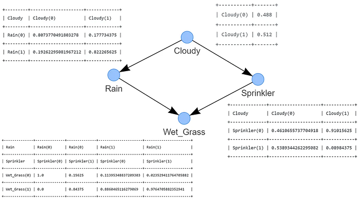
Computing the CPTs manually using MLE is straightforward; let me demonstrate this by example by computing the CPTs manually for the nodes Cloudy and Rain.

# Examples to illustrate how to manually compute MLE for the node Cloudy and Rain:

# Compute CPT for the Cloudy Node:
# This node has no conditional dependencies and can easily be computed as following:

# P(Cloudy=0)
sum(df['Cloudy']==0) / df.shape[0] # 0.488

# P(Cloudy=1)
sum(df['Cloudy']==1) / df.shape[0] # 0.512

# Compute CPT for the Rain Node:
# This node has a conditional dependency from Cloudy and can be computed as following:

# P(Rain=0 | Cloudy=0)
sum( (df['Cloudy']==0) & (df['Rain']==0) ) / sum(df['Cloudy']==0) # 394/488 = 0.807377049

# P(Rain=1 | Cloudy=0)
sum( (df['Cloudy']==0) & (df['Rain']==1) ) / sum(df['Cloudy']==0) # 94/488  = 0.192622950

# P(Rain=0 | Cloudy=1)
sum( (df['Cloudy']==1) & (df['Rain']==0) ) / sum(df['Cloudy']==1) # 91/512  = 0.177734375

# P(Rain=1 | Cloudy=1)
sum( (df['Cloudy']==1) & (df['Rain']==1) ) / sum(df['Cloudy']==1) # 421/512 = 0.822265625

Note that conditional dependencies can be based on limited data points. As an example, P(Rain=1|Cloudy=0) is based on 91 observations. If Rain had more than two states and/or more dependencies, this number would have been even lower. Is more data the solution? Maybe. Maybe not. Just keep in mind that even if the total sample size is very large, the fact that state counts are conditional for each parent's configuration can also cause fragmentation. Check out the differences between the CPTs compared to the MLE approach.

# Parameter learning on the user-defined DAG and input data using Bayes
model_bayes = bn.parameter_learning.fit(DAG, df, methodtype='bayes')

# Print the learned CPDs
bn.print_CPD(model_bayes)

"""
[bnlearn] >Compute structure scores for model comparison (higher is better).
[bnlearn] >[Conditional Probability Table (CPT)] >[Node Sprinkler]:
+--------------+--------------------+--------------------+
| Cloudy       | Cloudy(0)          | Cloudy(1)          |
+--------------+--------------------+--------------------+
| Sprinkler(0) | 0.4807692307692308 | 0.7075098814229249 |
+--------------+--------------------+--------------------+
| Sprinkler(1) | 0.5192307692307693 | 0.2924901185770751 |
+--------------+--------------------+--------------------+

[bnlearn] >[Conditional Probability Table (CPT)] >[Node Rain]:
+---------+--------------------+---------------------+
| Cloudy  | Cloudy(0)          | Cloudy(1)           |
+---------+--------------------+---------------------+
| Rain(0) | 0.6518218623481782 | 0.33695652173913043 |
+---------+--------------------+---------------------+
| Rain(1) | 0.3481781376518219 | 0.6630434782608695  |
+---------+--------------------+---------------------+

[bnlearn] >[Conditional Probability Table (CPT)] >[Node Wet_Grass]:
+--------------+--------------------+-----+---------------------+
| Rain         | Rain(0)            | ... | Rain(1)             |
+--------------+--------------------+-----+---------------------+
| Sprinkler    | Sprinkler(0)       | ... | Sprinkler(1)        |
+--------------+--------------------+-----+---------------------+
| Wet_Grass(0) | 0.7553816046966731 | ... | 0.37910447761194027 |
+--------------+--------------------+-----+---------------------+
| Wet_Grass(1) | 0.2446183953033268 | ... | 0.6208955223880597  |
+--------------+--------------------+-----+---------------------+

[bnlearn] >[Conditional Probability Table (CPT)] >[Node Cloudy]:
+-----------+-------+
| Cloudy(0) | 0.494 |
+-----------+-------+
| Cloudy(1) | 0.506 |
+-----------+-------+

[bnlearn] >Independencies:
(Rain ⟂ Sprinkler | Cloudy)
(Sprinkler ⟂ Rain | Cloudy)
(Wet_Grass ⟂ Cloudy | Rain, Sprinkler)
(Cloudy ⟂ Wet_Grass | Rain, Sprinkler)
[bnlearn] >Nodes: ['Cloudy', 'Sprinkler', 'Rain', 'Wet_Grass']
[bnlearn] >Edges: [('Cloudy', 'Sprinkler'), ('Cloudy', 'Rain'), ('Sprinkler', 'Wet_Grass'), ('Rain', 'Wet_Grass')]
"""

Inferences.

Making inferences requires the Bayesian network to have two main components: A Directed Acyclic Graph (DAG) that describes the structure of the data and Conditional Probability Tables (CPT) that describe the statistical relationship between each node and its parents. At this point, you have the data set, you computed the DAG using structure learning, and estimated the CPTs using parameter learning. You can now make inferences! For more details about inferences, I recommend reading this blog:

With inferences, we marginalize variables in a procedure that is called variable elimination. Variable elimination is an exact inference algorithm. It can also be used to figure out the state of the network that has maximum probability by simply exchanging the sums by max functions. Its downside is that for large BNs, it might be computationally intractable. Approximate inference algorithms such as Gibbs sampling or rejection sampling might be used in these cases [7]. See the code block below to make inferences and answer questions like:

How probable is it to have wet grass given that the sprinkler is off?

import bnlearn as bn

# Load sprinkler data set
df = bn.import_example('sprinkler')

# Define the causal dependencies based on your expert/domain knowledge.
# Left is the source, and right is the target node.
edges = [('Cloudy', 'Sprinkler'),
         ('Cloudy', 'Rain'),
         ('Sprinkler', 'Wet_Grass'),
         ('Rain', 'Wet_Grass')]

# Create the DAG
DAG = bn.make_DAG(edges)

# Parameter learning on the user-defined DAG and input data using Bayes to estimate the CPTs
model = bn.parameter_learning.fit(DAG, df, methodtype='bayes')
bn.print_CPD(model)

q1 = bn.inference.fit(model, variables=['Wet_Grass'], evidence={'Sprinkler':0})
[bnlearn] >Variable Elimination.
+----+-------------+----------+
|    |   Wet_Grass |        p |
+====+=============+==========+
|  0 |           0 | 0.486917 |
+----+-------------+----------+
|  1 |           1 | 0.513083 |
+----+-------------+----------+

Summary for variables: ['Wet_Grass']
Given evidence: Sprinkler=0

Wet_Grass outcomes:
- Wet_Grass: 0 (48.7%)
- Wet_Grass: 1 (51.3%)

The Answer to the question is: P(Wet_grass=1 | Sprinkler=0) = 0.51. Let's try another one:

How probable is it to have rain given sprinkler is off and it is cloudy?

q2 = bn.inference.fit(model, variables=['Rain'], evidence={'Sprinkler':0, 'Cloudy':1})
[bnlearn] >Variable Elimination.
+----+--------+----------+
|    |   Rain |        p |
+====+========+==========+
|  0 |      0 | 0.336957 |
+----+--------+----------+
|  1 |      1 | 0.663043 |
+----+--------+----------+

Summary for variables: ['Rain']
Given evidence: Sprinkler=0, Cloudy=1

Rain outcomes:
- Rain: 0 (33.7%)
- Rain: 1 (66.3%)

The Answer to the question is: P(Rain=1 | Sprinkler=0, Cloudy=1) = 0.663. Inferences can also be made for multiple variables; see the code block below.

How probable is it to have rain and wet grass given sprinkler is on?

# Inferences with two or more variables can also be made such as:
q3 = bn.inference.fit(model, variables=['Wet_Grass','Rain'], evidence={'Sprinkler':1})
[bnlearn] >Variable Elimination.
+----+-------------+--------+----------+
|    |   Wet_Grass |   Rain |        p |
+====+=============+========+==========+
|  0 |           0 |      0 | 0.181137 |
+----+-------------+--------+----------+
|  1 |           0 |      1 | 0.17567  |
+----+-------------+--------+----------+
|  2 |           1 |      0 | 0.355481 |
+----+-------------+--------+----------+
|  3 |           1 |      1 | 0.287712 |
+----+-------------+--------+----------+

Summary for variables: ['Wet_Grass', 'Rain']
Given evidence: Sprinkler=1

Wet_Grass outcomes:
- Wet_Grass: 0 (35.7%)
- Wet_Grass: 1 (64.3%)

Rain outcomes:
- Rain: 0 (53.7%)
- Rain: 1 (46.3%)

The Answer to the question is: P(Rain=1, Wet grass=1 | Sprinkler=1) = 0.287712.

How do I know my causal model is right?

When a causal diagram is derived solely from data, it is difficult to fully verify its validity and completeness. Like any model, causal networks are subject to variation depending on the chosen approach (e.g., scoring or search algorithms), which may produce different structures. Still, there are ways to build confidence in your model. One option is to empirically test conditional independence (or dependence) relationships between variables — if these are absent in the data, it can indicate the model's correctness [8]. Another option is to incorporate prior expert knowledge, such as predefined DAGs or conditional probability tables (CPTs), to strengthen trust in the model's inferences.

Discussion

In this article, I touched on the concepts of why correlation and association is not causation and how to go from data towards a causal model using structure learning. A summary of the advantages of Bayesian techniques are:

1. The outcome of posterior probability distributions, or the graph, allows the user to make a judgment on the model predictions instead of having a single value as an outcome.
2. The possibility of incorporating domain/expert knowledge in the DAG and reasoning with incomplete information and missing data. This is possible because Bayes' theorem is built on updating the prior term with evidence.
3. It has a notion of modularity, which enables making a complex system using simpler parts.
4. Graph theory provides intuitively highly interacting sets of variables.
5. Probability theory provides the glue to combine the parts.

A weakness of Bayesian networks is that finding the optimum DAG is computationally expensive since an exhaustive search over all the possible structures must be performed. The limit of nodes for exhaustive search can already be around 15 nodes, but it also depends on the number of states. In case you have a large data set with many nodes, you may want to consider alternative methods and define the scoring function and search algorithm. For very large data sets, those with hundreds or maybe even thousands of variables, tree-based or constraint-based approaches are often necessary with the use of black/whitelisting of variables. Such an approach first determines the order and then finds the optimal BN structure for that ordering. Determining causality can be a challenging task, but the bnlearn library is designed to tackle some of the challenges!

Be safe. Stay frosty.

Cheers, E.

I hope you enjoyed reading this article! You are welcome to follow me because I write more about Bayesian statistics! I recommend experimenting with the hands-on examples in this blog. This will help you to learn quicker, understand better, and remember longer. Grab a coffee and have fun!

Software

• Bnlearn Github
• Bnlearn Colab Notebook examples

Let's connect!

• Let's connect on LinkedIn
• Follow me on Github
• Follow me on Medium

References

1. McLeod, S. A, Correlation definitions, examples & interpretation. Simply Psychology, 2018, January 14
2. F. Dablander, An Introduction to Causal Inference, Department of Psychological Methods, University of Amsterdam, https://psyarxiv.com/b3fkw
3. Brittany Davis, When Correlation is Better than Causation, Medium, 2021
4. Paul Gingrich, Measures of association. Page 766–795
5. E. Taskesen, Uncover Hidden Patterns In Your Tabular Datasets: All You Need Is The Right Statistics., Data Science Collective (DSC), June 2025
6. Branislav Holländer, Introduction to Probabilistic Graphical Models, Medium, 2020
7. Harini Padmanaban, Comparative Analysis of Naive Analysis of Naive Bayes and Tes and Tree Augmented Naive augmented Naive Bayes Models, San Jose State University, 2014
8. Huszar. F, ML beyond Curve Fitting: An Intro to Causal Inference and do-Calculus
9. AI4I 2020 Predictive Maintenance Data set. (2020). UCI Machine Learning Repository. Licensed under a Creative Commons Attribution 4.0 International (CC BY 4.0).
10. E. Perrier et al, Finding Optimal Bayesian Network Given a Super-Structure, Journal of Machine Learning Research 9 (2008) 2251–2286.
11. E. Taskesen, Synthetic Data: The Essentials Of Data Generation Using Bayesian Sampling., Data Science Collective (DSC), May 2025
12. E. Taskesen, Why Prediction Isn't Enough: Using Bayesian Models to Change the Outcome., Towards Data Science (TDS), June 2025