LLMs for Causal Discovery

Incorporating Expert Knowledge for Improved Causal Discovery

An iterative causal discovery algorithm that integrates expert knowledge or large language models to refine DAGs, reducing errors common in purely data-driven approaches

Causal discovery is a challenging task in causal inference. Causal discovery methods aim to identify causal relationships between variables, typically represented as a Directed Acyclic Graph (DAG). These graphs can be used for understanding the cause-and-effect relationship between the variables, but the challenge lies in accurately constructing them from observational data alone. Users often rely on domain expertise to either manually construct the model or correct/modify models generated by an algorithm. In this post, we will explore pgmpy's Expert-In-The-Loop causal discovery algorithm, which iteratively asks for expert knowledge from the user to construct the DAG. In the absence of an expert, a large language model (LLM) can also be used.

Problems with Causal Discovery Algorithms

Many automated causal discovery algorithms have been proposed with strong asymptotic properties. However, applying these algorithms to real finite-size datasets can present several problems:

1. Obvious Mistakes: In finite sample scenarios, these algorithms often make obvious mistakes, making it difficult to trust the algorithm's output. Additionally, the outputs can vary significantly depending on the chosen algorithm and its hyperparameters.
2. Markov Equivalence Class (MEC): Often, multiple DAGs can represent the same observed dataset, causing the algorithm to learn the MEC, which represents a set of all such DAGs. However, most methods for downstream tasks, such as causal identification or effect estimation, assume knowledge of a single DAG.

As a result of these issues, users often have to rely on their expert knowledge to correct the algorithm's mistakes and select the most appropriate DAG from the MEC.

Examples

To highlight some of these issues, we can take an example using the Adult Income dataset (also known as the Census Income dataset)[1] and attempt to learn the DAG from it using two of the most commonly used causal discovery algorithms: the PC algorithm[2] and the Hill Climb Search algorithm[3].

Firstly, we start by preprocessing the data and define the correct variable types. Some of the variables in the dataset are ordinal (i.e., ordered categorical) and other are categorical.

df = pd.read_csv("https://raw.githubusercontent.com/pgmpy/pgmpy/refs/heads/dev/pgmpy/tests/test_estimators/testdata/adult_proc.csv", index_col=0)
df.Age = pd.Categorical(
    df.Age,
    categories=["<21", "21-30", "31-40", "41-50", "51-60", "61-70", ">70"],
    ordered=True,
)
df.Education = pd.Categorical(
    df.Education,
    categories=[
        "Preschool",
        "1st-4th",
        "5th-6th",
        "7th-8th",
        "9th",
        "10th",
        "11th",
        "12th",
        "HS-grad",
        "Some-college",
        "Assoc-voc",
        "Assoc-acdm",
        "Bachelors",
        "Prof-school",
        "Masters",
        "Doctorate",
    ],
    ordered=True,
)
df.HoursPerWeek = pd.Categorical(
    df.HoursPerWeek, categories=["<=20", "21-30", "31-40", ">40"], ordered=True
)
df.Workclass = pd.Categorical(df.Workclass, ordered=False)
df.MaritalStatus = pd.Categorical(df.MaritalStatus, ordered=False)
df.Occupation = pd.Categorical(df.Occupation, ordered=False)
df.Relationship = pd.Categorical(df.Relationship, ordered=False)
df.Race = pd.Categorical(df.Race, ordered=False)
df.Sex = pd.Categorical(df.Sex, ordered=False)
df.NativeCountry = pd.Categorical(df.NativeCountry, ordered=False)
df.Income = pd.Categorical(df.Income, ordered=False)

We can now use the preprocessed data to learn the DAG using PC and Hill-Climb Search algorithms.

from pgmpy.estimators import PC

est_pc = PC(df)
cpdag_pillai = est_pc.estimate(ci_test="pillai", return_type="cpdag")
cpdag_pillai.to_graphviz().draw("adult_pillai.png", prog="dot")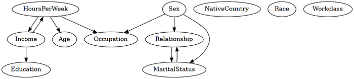

from pgmpy.estimators import HillClimbSearch

est_hill = HillClimbSearch(df)
dag_hill = est_hill.estimate(scoring_method="bic-d")
dag_hill.to_graphviz().draw("adult_hill.png", prog="dot")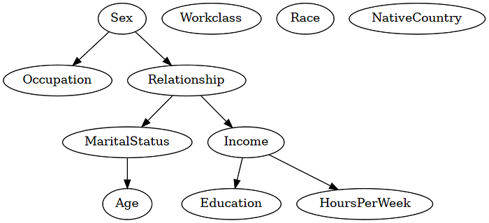

As we can see from the output of both these algorithms, the learned graphs have a few incorrect edges. For example, in the dataset, we would expect an edge Workclass -> Income, which both the algorithms missed. We would also expect an edge from Education -> Income, which both the algorithms got wrong. Moreover, as both these algorithms can only learn the MEC, there are some undirected (represented using bi-directed edges) in the model.

Expert-In-The-Loop Causal Discovery

Instead of users utilizing their expertise to make post-hoc modifications or orientating edges of the learned model, the Expert-In-The-Loop causal discovery algorithm[4] iteratively asks for expert knowledge and incorporates that into the model-building process. The algorithm is similar to the Greedy Equivalence Search and works as follows:

1. Start with an empty graph.
2. In each iteration, run a conditional independence test and compute the partial association between each pair of variables.
3. Remove any edges that have a p-value above the threshold and a partial association below the threshold.
4. Among the edge pairs that have a p-value below the threshold and partial association above the threshold, use a greedy approach to adds an edge between them. The orientation of the edge is determined using expert knowledge.
5. Repeat Steps 2–4 until no more edges can be added or removed.

The user can provide expert knowledge manually or we can use an LLM.

Using LLM for Expert Knowledge

When using an LLM as the expert, the algorithm requires textual descriptions of the variables that it uses to query the LLM for the edge orientation between them. Following is an example of applying this algorithm to the Adult Income dataset.

from pgmpy.estimators import ExpertInLoop

descriptions = {
    "Age": "The age of a person",
    "Workclass": "The workplace where the person is employed such as ",
       "Private industry, or self employed",
    "Education": "The highest level of education the person has finished",
    "MaritalStatus": "The marital status of the person",
    "Occupation": "The kind of job the person does. For example, sales, craft repair, ",
        "clerical",
    "Relationship": "The relationship status of the person",
    "Race": "The ethnicity of the person",
    "Sex": "The sex or gender of the person",
    "HoursPerWeek": "The number of hours per week the person works",
    "NativeCountry": "The native country of the person",
    "Income": "The income i.e. amount of money the person makes",
}

estimator = ExpertInLoop(df)
dag = estimator.estimate(pval_threshold=0.05,
                         effect_size_threshold=0.05,
                         variable_descriptions=descriptions,
                         use_llm=True,
                         llm_model="gemini/gemini-1.5-flash")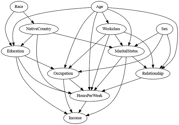

As we see from this learned graph, it is able to directly learn a DAG by utilizing expert knowledge to orient the edges. Moreover, it doesn't make as many mistakes as the other algorithms. We can see that many of the edges that were incorrect in the PC and Hill Climb Search algorithm are correct in this case, such as Education -> Income, HoursPerWeek -> Income, and Occupation -> Income.

Specifying Expert Knowledge Manually

We can also manually provide the required edge orientations instead of using an LLM. If the use_llm=False argument is passed, the method then iteratively prompts the user to provide the orientation of the edge.

from pgmpy.estimators import ExpertInLoop

estimator = ExpertInLoop(df)
dag = estimator.estimate(pval_threshold=0.05,
                         effect_size_threshold=0.05,
                         use_llm=False)
Select the edge direction between MaritalStatus and Relationship. 
 1. MaritalStatus -> Relationship 
 2. MaritalStatus <- Relationship 
1
Select the edge direction between Education and NativeCountry. 
 1. Education -> NativeCountry 
 2. Education <- NativeCountry 
2

Controlling Model Density

To control the edge density in the learned model, we can use the pval_threshold and effect_size_threshold arguments. Similar to constraint-based algorithms like PC, increasing the p-value threshold results in denser graphs, while increasing the effect_size_threshold results in sparser graphs.

References

[1] https://archive.ics.uci.edu/dataset/2/adult

[2] https://pgmpy.org/structure_estimator/pc.html

[3] https://pgmpy.org/structure_estimator/hill.html

[4] https://pgmpy.org/structure_estimator/expert.html