The Starters Guide To Learn Generating Synthetic Data: Sampling From Univariate Distributions

Learn how to generate synthetic data when real-world data is scarce or when only expert knowledge is available. A practical guide combining theory, code, and real applications.

Data is the fuel in Data Science projects. But what if the observations are scarce, expensive, or difficult to measure? Synthetic data can be the solution. Synthetic data is artificially generated data that mimics the statistical properties of real-world events. In this blog, you will learn how to generate continuous synthetic data by sampling from univariate distributions. First, we will go through probability distributions on how to specify the parameters to generate synthetic data. After that, we will generate data that mimics the properties of an existing data set, i.e., the random variables that are distributed according to a probabilistic model. All examples are created using scipy and the distfit library.

If you like the content, give it a few claps! You are welcome to follow me because I write more about data science. Tip: Try the hands-on examples in this blog. This will help you to learn quicker, understand better, and remember longer. Grab a coffee and have fun!

Synthetic Data — Background.

In the last decade, the amount of data has grown rapidly and led to the insight that higher-quality data is more important than simply having more data. Higher quality can help to draw more accurate conclusions and better-informed decisions. There are many organizations and domains where synthetic data can be of use, but there is one in particular that is heavily invested in synthetic data, namely, for autonomous vehicles. Here, data is generated for many edge cases that are subsequently used to train models. The importance of synthetic data is stressed by companies like Gartner, which predicts that real data will be overshadowed in the coming years [1]. Clear examples are already all around us, such as images generated by Generative Adversarial Networks (GANs). In this blog, I will not focus on images produced by GANs but instead focus on the more fundamental techniques, i.e., creating synthetic data based on probability distributions.

In general, synthetic data can be created across two broad categories:

1. Probability sampling: Create synthetic data that closely mirrors the distribution of the real data, making it useful for training machine learning models and performing statistical analysis.
2. Non-probability sampling: Involves selecting samples without a known probability of selection, such as convenience sampling, snowball sampling, and quota sampling. It is a fast, easy, and inexpensive way of obtaining data.

I will focus on probability sampling, in which estimating the distribution parameters of the population is key. Or in other words, we search for the best-fitting theoretical distribution in the case of univariate data sets. With the estimated theoretical distribution, we can then generate new samples, our synthetic data set.

Overview of probability density functions.

Finding the best-fitting theoretical distribution that mimics real-world events can be challenging, as there are many different probability distributions. Libraries such as distfit [2] are very helpful in such cases. For more details, I recommend reading this blog.

A great overview of Probability Density Functions (PDF) is shown in Figure 1 where the "canonical" shapes of the distributions are captured. Such an overview can help to better understand and decide which distribution may be most appropriate for a specific use case. In the following two sections, we will experiment with different distributions and their parameters and see how well we can generate synthetic data.

Synthetic data is artificial data generated using statistical models.

Create Synthetic Data Based on Expert Knowledge.

The use of synthetic data is ideal to generate large and diverse datasets for, among others, simulation purposes because it can help in testing and exploring different scenarios. As an example, certain edge cases may be difficult (or too dangerous) to obtain in practical situations. To demonstrate how to design a system that can generate synthetic data, I will use a hypothetical use case in the security domain. This could have been any other domain, but the point that I want to demonstrate is how to translate expert knowledge into a model that can then be used to generate synthetic data.

With synthetic data we aim to mimick real-world events by estimating theoretical distributions, and population parameters.

Suppose you are a data scientist working together with security experts. The network activity behavior needs to be analyzed and understood, and a security expert provided you with the following information:

1. Most network activities start at 8 and peak around 10.
2. Some activities will be seen before 8 but not a lot.
3. In the afternoon, the activities gradually decrease and stop around 6 pm.
4. Usually, there is a small peak at 1–2 pm too.

Note that in general, it is much harder to describe abnormal events than what is normal/expected behavior because of the fact that normal behavior is most commonly seen and thus the largest proportion of the observations. In the following two subsections, we will translate this information into a probabilistic model.

Step 1. Translate domain knowledge into a statistical model.

With the description, we need to decide the best-matching theoretical distribution. However, choosing the best theoretical distribution requires investigating the properties of many distributions (see Figure 1). In addition, you may need more than one distribution; namely, a mixture of probability density functions. In our example, we will create a mixture of two distributions, one PDF for the morning and one PDF for the afternoon activities.

Description morning: "Most network activities start at 8 and peak around 10. Some activities will be seen before 8 but not a lot."

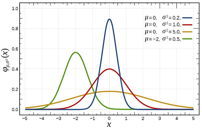
To model the morning network activities, we can use the Normal distribution. It is symmetrical and has no heavy tails. We can set the following parameters; a mean of 10 am and a relatively narrow spread, such as sigma=0.5. In Figure 2 is shown A few normal PDFs with different mu and sigma parameters. Try to get feeling how the slope changes on the sigma parameter.

Decription afternoon: "The activities gradually decrease and stop arround 6 pm. However, there is a small peak at 1–2 pm too."

A suitable distribution for the afternoon activities could be a skewed distribution with a heavy right tail that can capture the gradual decreasing activities. The Weibull distribution can be a candidate as it is used to model data that has a monotonic increasing or decreasing trend. However, if we do not always expect a monotonic decrease in network activity (because it is different on Tuesdays or so) it may be better to consider a distribution such as gamma (Figure 3). Here we need to tune the parameters too so that it best matches with the description. To have more control of the shape of the distribution, I prefereably use the generalized gamma distribution.

In the next section, we will use these model distributions and examine the parameters for the Normal and generalized Gamma distributions. We will also set parameters to create a mixture of PDFs that is representative of the use case of network activities.

2. Optimize parameters to create Synthetic data that best matches the scenario.

In this section, we will generate 10.000 samples from a normal distribution with a mean of 10 (representing the peak at 10 am) and a standard deviation of 0.5. Next, we generate 2000 samples from a generalized gamma distribution for which I set the second peak at loc=13. We could also have chosen loc=14, but that resulted in a larger gap between the two distributions. The next step is to combine the two datasets and shuffle them. Note that shuffling is not required, but without it, samples are ordered first by the 10.000 samples from the normal distribution and then by the 1000 samples from the generalized gamma distribution. This order could introduce bias in any analysis or modeling that is performed on the data set when splitting the data set.

import numpy as np
from scipy.stats import norm, gengamma
import matplotlib.pyplot as plt

# Set seed for reproducibility
np.random.seed(1)

# Generate data from a normal distribution
normal_samples = norm.rvs(10, 1, 10000)
# Create a generalized gamma distribution with the specified parameters
dist = gengamma(a=1.4, c=1, scale=0.8, loc=13)
# Generate random samples from the distribution
gamma_samples = dist.rvs(size=2000)
# Combine the two datasets by concatenation
dataset = np.concatenate((normal_samples, gamma_samples))
# Shuffle the dataset
np.random.shuffle(dataset)
# Plot
bar_properties={'color': '#607B8B', 'linewidth': 1, 'edgecolor': '#5A5A5A'}
plt.figure(figsize=(20, 15)); plt.hist(dataset, bins=100, **bar_properties)
plt.grid(True)
plt.xlabel('Time', fontsize=22)
plt.ylabel('Frequency', fontsize=22)Let's plot the distribution and see what it looks like (Figure 3). Usually, it takes a few iterations to tweak parameters and fine-tuning.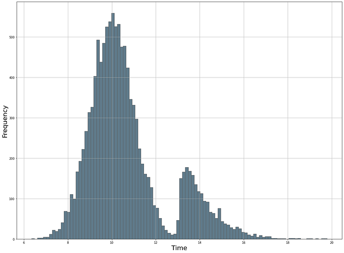

At this point, we created synthetic data using a mixture of two distributions to model the normal/expected behavior of network activity for a specific population (Figure 4). We modeled a major peak at 10 am with network activities starting from 6 am up to 1 pm. A second peak is modeled around 1–2 pm with a heavy right tail towards 8 pm. The next step could be setting the confidence intervals and pursuing the detection of outliers. For more details about outlier detection, I recommend reading the following blog [3]:

Creating Synthetic Data that Closely Mirrors the Distribution of Real Data.

Up to this point, we have created synthetic data that allows for exploring different scenarios using experts' knowledge. Here, we will create synthetic data that closely mirrors the distribution of real data. For demonstration, I will use the money tips dataset from Seaborn [4] and estimate the parameters using the distfit library [2]. I recommend reading the blog about distfit if you are new to estimating probability density functions. The tips data set contains only 244 data points. Let's first load the data set and plot the values (see code section below).

# Install distfit
pip install distfit
# Load library
from distfit import distfit

# Initialize distfit
dfit = distfit(distr='popular')

# Import dataset
df = dfit.import_example(data='tips')
print(df)
#        tip
# 0      1.01
# 1      1.66
# 2      3.50
# 3      3.31
# 4      3.61
# 239    5.92
# 240    2.00
# 241    2.00
# 242    1.75
# 243    3.00
# Name: tip, Length: 244, dtype: float64

# Make plot
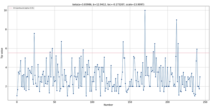
dfit.lineplot(df['tip'], xlabel='Number', ylabel='Tip value')

Visual inspection of the data set.

After loading the data, we can make a visual inspection to get a better intuition of the range and possible outliers (Figure 5). The range across the 244 tips is mainly between 2 and 4 dollars. Based on this plot, we can also build an intuition of the expected distribution when we project all data points toward the y-axis (I will demonstrate this later on).

The search space of distfit is set to the popular PDFs, and the smoothing parameter is set to 3. Low sample sizes can make the histogram bumpy and can cause poor distribution fits.

# Import library
from distfit import distfit

# Initialize with smoothing and upperbound confidence interval
dfit = distfit(smooth=3, bound='up')
# Fit model
dfit.fit_transform(df['tip'], n_boots=100)
# Plot PDF/CDF
fig, ax = plt.subplots(1,2, figsize=(25, 10))
dfit.plot(chart='PDF', n_top=10, ax=ax[0])
dfit.plot(chart='CDF', n_top=10, ax=ax[1])
# Show plot
plt.show()
# Create line plot
dfit.lineplot(df['tip'], xlabel='Number', ylabel='Tip value', projection=True)

The best-fitting PDF is beta (Figure 6, red line). The upper bound confidence interval alpha=0.05 is 5.53, which seems a reasonable threshold based on a visual inspection (red vertical line).

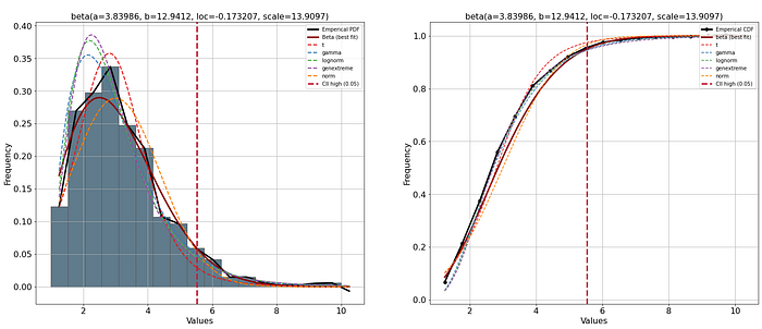
After finding the best distribution, we can project the estimated PDF on top of our line plot for better intuition (Figure 7). Note that both PDF and empirical PDF are the same as in Figure 6.

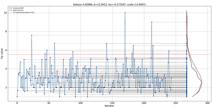
With the estimated parameters for the best-fitting distribution, we can start creating synthetic data for money tips (see code section below). Let's create 100 new samples and plot the data points (Figure 8). The synthetic data provides many opportunities, i.e., it can be used for training models, but also to get insights into questions such as the time it would take to save a certain amount of money using tips.

# Create synthetic data
X = dfit.generate(100)

# Ploy the data
dfit.lineplot(X, xlabel='Number', ylabel='Tip value', grid=True)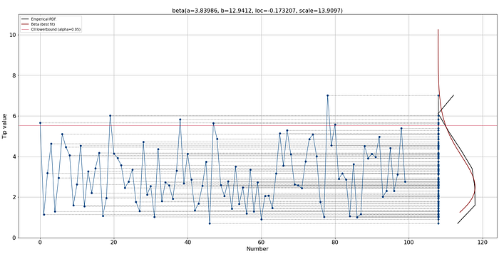

Final words.

I showed how to create synthetic data in a univariate manner by using probability density functions. With the distfit library, over 90 theoretical distributions can be evaluated, and the estimated parameters can be used to mimic real-world events. Although this is great, there are also some limitations in creating synthetic data. First, synthetic data may not fully capture the complexity of real-world events, and the lack of diversity can cause that models may not generalize when used for training. In addition, there is a possibility of introducing bias into the synthetic data because of incorrect assumptions or parameter estimations. Make sure to always perform sanity checks on your synthetic data.

Be Safe. Stay Frosty.

Cheers, E.

If you like the content, give it a few claps! You are welcome to follow me because I write more about data science. Tip: Try the hands-on examples in this blog. This will help you to learn quicker, understand better, and remember longer. Grab a coffee and have fun!

Software

• Distfit Github/Documentation
• Distfit notebook examples

Let's connect!

• Let's connect on LinkedIn
• Follow me on Github
• Follow me on Medium

References

1. Gartner, Maverick Research: Forget About Your Real Data — Synthetic Data Is the Future of AI, Leinar Ramos, Jitendra Subramanyam, 24 June 2021.
2. E. Taskesen, How to Find the Best Theoretical Distribution for Your Data, Data Science Collective (DSC), June 2025
3. E. Taskesen, Outlier Detection Using Distribution Fitting in Univariate Datasets, Data Science Collective (DSC), August 2025
4. Michael Waskom, Seaborn, Tips Data set, BSD-3 License